Hardware Architecture for Packet Classification with Prefix ... - VUT FIT

Hardware Architecture for Packet Classification with Prefix Coloring Viktor Puˇs, Michal Kajan, Jan Koˇrenek Faculty of Information Technology Brno University of Technology Boˇzetˇechova 2, Brno, Czech Republic Email: ipus,ikajan,[email protected]

Abstract—Packet classification is a widely used operation in network security devices. As network speeds are increasing, the demand for hardware acceleration of packet classification in FPGAs or ASICs is growing. Nowadays algorithms implemented in hardware can achieve multigigabit speeds, but suffer with great memory overhead. We propose a new algorithm and hardware architecture which reduces memory requirements of decomposition based methods for packet classification. The algorithm uses prefix coloring to reduce large amount of Cartesian product rules at the cost of an additional pipelined processing and a few bits added into results of the longest prefix match operation. The proposed hardware architecture is designed as a processing pipeline with the throughput of 266 million packets per second using commodity FPGA and one external memory. The greatest strength of the algorithm is the constant time complexity of the search operation, which makes the solution resistant to various classes of network security attacks.

proposed reduction significantly decreases overhead given by the Cartesian product nature of classification rules at the cost of additional pipelined processing which is performed by only small amount of logic resources. The rest of the paper is organized as follows: in the next section we discuss the related work and explain the reason of the excessive memory overhead. Section III introduces our new method of lowering memory overheads of these algorithms, as well as a proposed architecture of the whole packet classification algorithm. We provide a detailed example of algorithm function in section IV. Experimental results of our work are summed up in Section VI and Section VII concludes the paper.

I. I NTRODUCTION

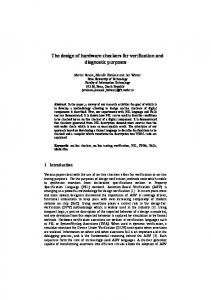
The simplest classification scheme uses only one packet header field. Packet routing in IP networks is a common example of one-dimensional classification (only destination IP address is important for routing). This search on prefixes is called the Longest Prefix Match (LPM) operation. From the given set of prefixes with various lengths, the LPM algorithm finds the one that best fits the given full-length value. This corresponds to both IPv4 and IPv6 addressing schemes. Because the LPM operation is performed in IP packet routing, it is well studied topic. Basic algorithm and data structure for the LPM is a trie – the tree algorithm processing one input bit at each tree level and returning the last valid prefix visited. Trie is often modified to process more input bits in each step and to reduce memory requirements. Popular examples of such algorithms are the Tree Bitmap [1] and the Shape Shifting Trie [2], both having a strong potential for hardware implementation. Fig. 1 shows an example of trie data structure for the longest prefix match operation. Black circles represent valid prefixes (possible results of LPM operation). From the wide choice of available algorithms for classification in multiple fields, we discuss those which are related to our work. All of them belong to the family of decompositionbased methods. We focus on these algorithms because of their potential to achieve the constant time complexity of the search operation. In decomposition methods, packet classification is divided into several steps (or pipeline stages in case of hardware implementation). Figure 2 shows the basic scheme of decomposition algorithms.

The growth of computer networks provides more opportunities for new applications and services, but also gives new possibilities for suspicious activities. Malicious traffic is usually detected by Intrusion Detection Systems (IDS) and then filtered by firewalls which performs per-packet classification based on the given set of rules. Packet classification is a problem of assigning each network packet into one or more classes. Classes are unambiguously determined by rules. Each rule defines a condition for all significant packet header fields (or dimensions). These fields are usually a 5-tuple (Source IP Address, Destination IP Address, Source Port, Destination Port, Protocol). A condition may be exact match, prefix match (usually for IP addresses), range match (for ports), or a wildcard, which matches any value. The goal of a packet classification algorithm is to find the matching rule with the highest priority. The output of the algorithm is the number of the matched rule. As network speeds are increasing, the demand for a high speed packet classification is also growing. Usually, constant time complexity is required in order to achieve wire speed processing and avoid vulnerability to attacks. Classification algorithms commonly use preprocessing of rules to create a data structure that supports high-speed searching. Nowadays algorithms and hardware architectures can achieve multigigabit speeds only at the cost of high memory requirements. We propose a novel method how to reduce memory requirements and still achieve high-speed packet classification. The

II. R ELATED WORK

1 0

1

10* 1

1

111*

0 1010* 1 10101

Fig. 1. Example of trie with four stored prefixes. Result for input 10100 will be 1010*. Packet ... Field n

Field 1 LPM

...

LPM LPM vector

Rule Search Rule number

Fig. 2.

Basic scheme of decomposition algorithms.

The input of packet classification is a vector of packet header fields. LPM operation is a first step which is performed for every packet header field independently. LPM is well studied and can be performed very fast: recently published approaches achieve billions of lookups per second using a dedicated hardware (ASIC or FPGA) [3]. Each LPM search engine returns one item from the prefix set, where prefix set is the set of all LPM results for the given ruleset and the given dimension. Result of the LPM Stage is the LPM vector, containing one prefix for each dimension. After the LPM, all fields of the resulting LPM vector must be processed in some way (this is specific for each algorithm) to get the correct rule number. Key issue is that the state space of LPM vectors can be extremely large. This is because all possible values of the LPM vector are obtained by creating the Cartesian product of prefix sets. One possible method of combining LPM results together is the Distributed Crossproducting of Field Labels [4]. LPM is modified to return all valid prefixes (not only the longest one) for the given field value. What follows is the hierarchical structure of small crossproduct engines. Inputs of each engine are two sets of prefixes (or Labels, in general). Engine then performs set membership query for each possible pair of Labels. Result of the engine is another set of Labels. The result of the last engine is in fact a set of rules, from which the one with the highest priority is selected. Multi Subset Crossproduct Algorithm [5] brings further improvements to decomposition methods. In this work, Dharmapurikar et al. replace Cartesian products by pseudorules. Because pseudorules expansion is still similar to Cartesian product, authors provide heuristics on how to break ruleset

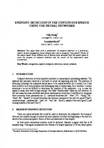
into several subsets, eliminating the majority of pseudorules. The paper also identifies rules that generate excessive amount of pseudorules. These rules are called spoilers and are treated in a separate algorithm branch (in hardware implementation, spoilers are moved to small on-chip TCAM) to further reduce number of pseudorules. The LPM operation is slightly modified to return a result for each subset, because subsets may contain different prefixes. A Bloom filter is associated with each subset to perform set membership query. If the Bloom filter output is true, one rule table memory access is performed to retrieve the resulting rule or pseudorule. We have recently published another Cartesian productbased approach: the Perfect Hashing Crossproduct Algorithm (PHCA) [6]. Our method uses specifically constructed hash function to map all pseudorules (in the form of LPM vectors) onto correct rules. This way, it is no longer necessary to store pseudorules, which saves a considerable amount of memory. The algorithm achieves high packet rate due to very simple Rule Search Stage. The processing time for each packet is guaranteed to be constant and PHCA is probably the first packet classification algorithm with constant time complexity of the search operation. However, the number of pseudorules affects the size of data structures of the hash function. This means that even this memory-optimized algorithm may be significantly improved if the number of pseudorules is reduced. The algorithms mentioned in this section achieve very good speeds in case of implementation in FPGA, but their memory requirements may be limiting and should be improved. Our current goal is to design a new algorithm inspired by previous Cartesian product-based algorithms. The two memory optimization techniques introduced in [5] (spoilers removal and use of subsets) are orthogonal to the method presented in this paper, which means that they are direct competition, but also that all memory reduction methods may be used together to produce even better results. III. M EMORY OPTIMIZATION We describe in detail how pseudorules are created and why this process increases the size of data structures in packet classification algorithms. To cover all valid combinations of LPM results, pseudorules must be added to the ruleset. In fact, a pseudorule is always a special case of some rule. This is best explained by the example of pseudorules generation in Fig. 3. We can see a simplified classification in two three-bit dimensions with three rules. In each dimension, trie is shown to illustrate the LPM operation. Colored arcs are the rules. For example, LPM vector for packet with header fields (111, 100) will be (1∗, 100). This combination is not in the original ruleset, but it is clear that the correct result is rule R1(1∗, ∗)1. Therefore, pseudorule P 1(1∗, 100) has to be added to handle this situation. Tab. I contains all rules and pseudorules together. Target rule in this table points to the correct classification result. 1 Symbol

* denotes prefix or wildcard

therefore LPM results table would use very wide data words. To illustrate sizes of bitmaps, we provide numbers of unique prefixes in each dimension for several real-life rulesets from university network firewalls (rules1-4), as well as synthetic rulesets generated by ClassBench [7] (synth1-2). ClassBench is a tool that produces synthetic rulesets that accurately model the characteristics of real rulesets. Basic properties of rulesets are shown in Tab. II.

Fig. 3.

Three rules R1, R2, R3 and three added pseudorules.

Rule R1 R2 R3 P1 P2 P3

Dimension 1 1* 1* 101 1* 101 101

Dimension 2 * 00* 100 100 00* *

Target rule R1 R2 R3 R1 R2 R1

Ruleset

Rules

synth1 synth2 rules1 rules2 rules3 rules4

219 394 103 173 275 1107

SRC IPs 55 65 28 84 46 158

DST IPs 53 57 48 84 64 80

Protocols 1 1 3 2 2 3

SRC Ports 13 13 5 1 1 1

DST Ports 1 1 39 15 17 55

TABLE II N UMBERS OF UNIQUE VALUES IN RULESETS .

TABLE I RULES AND PSEUDORULES .

The generation of pseudorules is similar to Cartesian product, and may potentially expand the ruleset significantly, but not all possible combinations of prefixes need to be added. If the universal rule (a rule covering all possible packets) was in the ruleset, then all possible combinations would have to be added. However, this rule can be removed from the ruleset and returned as a result only if no other rule matches the packet. Therefore, pseudorules are a subset of Cartesian product of all prefix sets. Let’s now focus on the fact that the LPM operation is performed independently for each field in decomposition-based packet classification algorithms (see Fig. 2). The advantage of this scheme is the strong potential for parallel computation. On the other hand, LPM results are logically related – only certain combinations of LPM results form a rule, the rest of them are unwished pseudorules. Thus, the knowledge of LPM result from one dimension should affect LPM result in other dimensions. A. Color Processing Stage Let’s suppose that the LPM operation is modified to return all matching prefixes, not only the longest one. Then, let each prefix P contain a precomputed bitmap for each of remaining dimensions. In the bitmap, there is one bit for each prefix. The bit corresponding to prefix R is set to 1, if prefixes P and R appear together in some rule. Otherwise, the bit is set to 0. This way, it is possible to remove almost all pseudorules easily by a simple logic, because each LPM result contains an information about ”allowed” and ”suppressed” prefixes from other dimensions. To be able to remove all pseudorules, information about rules priority would have to be attached. This approach has a disadvantage in adding large memory overhead to the LPM results. Number of prefixes may be large,

As can be seen, numbers of prefixes are prohibitive for perprefix bitmaps in bigger rulesets. Therefore, we will create groups of prefixes, and store only small bitmaps for these groups. We assign an abstract color property to each prefix. Number of colors is set to be much smaller than the number of prefixes. Instead of carrying large bitmaps of prefixes, each prefix contains its own color, and only a small bitmap of colors for each other dimension. We call this bitmap Allowed Colors Bitmap (ACB). Instead of returning all matching prefixes, the LPM operation returns the longest matching prefix for each color. Also, it returns the Aggregate Allowed Colors Bitmap (AACB) which is a bitwise logical disjunction (OR) of ACBs observed during the LPM tree descent. The Color Processing Stage is added after the LPM Stage. It performs the operations shown in Alg. 1. The method of assigning colors to prefixes is based on observation made by us and also other researchers [4], [8]: The number of prefixes matching a given value is small, typically less than five. To gain as much information as possible, it is good if each of prefixes returned by one LPM search has different color. Therefore, we assign numbers sequentially down the tree. If the number of colors does not suffice, the last color is repeated, because lower levels of tree usually do not generate greater amount of pseudorules. We continue to the method filling ACBs in prefixes: At the beginning, all bitmaps contain zeros. Then for each rule R and each prefix P of rule R, set bits in the ACB to one, such that bitmaps allow colors of all other prefixes of the rule R. It remains to find an algorithm that generates pseudorules. Thanks to colors and color bitmaps, majority of pseudorules will not exist in our algorithm. However, some pseudorules will be generated for most rulesets. Our experience with algorithms from Related work is that generating all pseudorules during the software precomputation phase may be very timeconsuming operation. Therefore it is undesirable to generate

Algorithm 1 Operations of the Color Processing Stage. Input: AACB for each dimension, prefix for each dimension and color. for all dimension d do create the Present Colors Bitmap (P CBd ) where bits correspond to colors in dimension d. Each bit is set to 1 if some prefix with that color was returned by the LPM, and to 0 otherwise. end for for all dimension d do Final Allowed Colors Bitmap F ACBd ← from bitwise and (P CBd , corresponding AACBs all other dimensions ). end for if some F ACB contained all zeros then Packet matches no rule. else Create empty output LPM vector V . for all dimension d do Add the longest matching prefix allowed by F ACBd to V . end for end if Output: V

all pseudorules and then remove some of them. Instead, we present an algorithm that directly generates only pseudorules that are really needed (Alg. 2).

Algorithm 2 Pseudorules generating with respect to colors. Input: Rules with prefixes containing ACBs and their own color. Create empty list of pseudorules P . The ruleset is traversed from the highest to lowest priority: for all rule R do for all dimension d do Ld ← list of all prefixes from dimension d matching the rule R. In this list, there is the prefix from the rule R, and all more specific (longer) prefixes from other rules. end for A decision tree is traversed. Each tree level corresponds to one dimension, dimension ordering is unimportant. Tree edges are prefixes from L. The tree is traversed by a depth-first traversal algorithm. Descent is performed only if colors and ACBs in prefixes allow the combination of prefixes from tree root to the current leaf. if the lowest tree level is reached then if the combination of prefixes from root to leaf ∈ / P then Add the prefix combination into P . (R is also added by this operation) end if end if end for Output: P

IV. C OLOR P ROCESSING E XAMPLE

B. Rule Search Stage We propose the Rule Search Stage to be the same as in our previous algorithm PHCA [6]: a special hash function mapping all rules and pseudorules directly onto correct rule number. Perfect hash function construction algorithm [9] is used to create the hash function. The perfect hash construction algorithm creates acyclic graph, where edges are the keys, and vertices are results of two different hash functions. Vertices are then assigned values so that they sum up to the desired hash value. In our algorithm, keys are rules and pseudorules in the form of LPM vectors, and associated numbers are numbers of the correct rule. This way, we get a function that hashes rule and all its associated pseudorules directly to the correct rule number. In fact, we introduce intended collisions of the hash function. The idea of intended hash collisions is a nontraditional usage of perfect hash functions. After the graph is created, the hash value computation is simple and well suitable for hardware implementation: At first, two ordinary hash functions f1 and f2 of the input LPM vector are computed. Then two vertex values are read from the Vertex Table and added. For each vertex, only one integer is stored. We propose the Vertex Table to be stored in offchip SRAM, while the rest of the algorithm be implemented in FPGA. The important point is that none of pseudorules is stored in our scheme. Therefore, we save significant amount of on-chip memory.

To demonstrate function of the algorithm, we use example ruleset from Fig. 3. Fig. 4 shows how colors are assigned to prefixes, and how the color bitmaps are filled. Bitmaps are shown as sets. Two colors are used in each dimension. Fig. 5 is a decision tree, according which the pseudorules are generated. In our example, one pseudorule is generated. Tree paths (f 1p2, f 2p1) and (f 1p2, f 2p2) are not examined, because prefix f 1p2 has color c1, and color bitmaps of prefixes f 2p1 and f 2p2 do not allow color c1. We continue by showing how a packet is processed. Suppose packet with header fields (101, 000). In the Field 1, the LPM returns: •

•

For each color, name and length of the longest matching prefix: c0 : (f 1p1, 0) and c1 : (f 1p2, 3). AACB gathered from visited prefixes: {d0, d1}

In the Field 2, the LPM returns: •

•

For each color, name and length of the longest matching prefix: d0 : (f 2p1, 0) and d1 : (f 2p2, 2). AACB gathered from visited prefixes: {c0}

The result in the Field 1 is f 1p1, because only color c0 is allowed by Field 2 results, and f 1p1 is the longest matching prefix of this color. The result in the Field 2 is f 2p2, because both colors d0 and d1 are allowed by Field 1 results, and f 2p2 is the longest matching prefix.

Prefix name = f2p1 Color = d0 Field 1 ACB = {c0}

Field 1

Software precomputation SRAM FPGA

Field 2 R1

SRC IP

1

Prefixes

CP

LPM

Universal rule

CB AA

0

1 0

0 0

1 P1

DST IP

SRC Port

DST Port

Protocol

LPM LPM

Prefix name = f2p2 Color = d1 Field 2 ACB = {c0}

CP

LPM

Prefix colors and color bitmaps.

LPM vector

Fig. 6. FPGA architecture. CP blocks are parts of the Color Processing Stage, shown in detail in the following Fig. Color 0 prefix Color 0 length Color 0 valid

Find longest allowed

...

Fig. 4.

Rule Check

h2

R3 Prefix name = f2p3 Color = d1 Field 1 ACB = {c1}

Rule Table

+

LPM

FIFO

Prefix name = f1p2 Color = c1 Field 2 ACB = {d1}

Rule number

h1 ...

R2

0

Data

Address

AA AAC AA CB CB B

Prefix name = f1p1 Color = c0 Field 2 ACB = {d0, d1}

Color C-1 prefix Color C-1 length Color C-1 valid PCB

...

Dimension 1 AACB

&

FACB

Dimension D-1 AACB

Fig. 7. Color processing in dimension 0 (supposing C colors and D dimensions). Fig. 5.

Decision tree for generating pseudorules.

To sum up the example, our prefix colors and color bitmaps avoided unwanted combination of LPM results (f 1p2, f 2p2), which would be returned in case of unmodified LPM operation. Instead, combination (f 1p1, f 2p2) is the output of the Color Processing Stage.

in each dimension. Because MSCA, PHCA and PCCA use LPM as a first stage, we do not compare LPM operation implementation, we only measure memory added to LPM results by each algorithm (Tab III, DCFL algorithm is not shown because it has no separate LPM Stage). In Tab. IV we measure amount of memory needed to implement the Rule Search Stage.

V. A RCHITECTURE The algorithm is by design targeted to use FPGA to implement required logic and one external SRAM with only narrow data bus (see Sec. VI-B) to store the data for the perfect hash function. Software precomputation and filling of memories is used for the architecture initialization. The architecture is shown in Fig. 6, while one part of the Color Processing Stage is shown in more detail in Fig. 7.

Ruleset synth1 synth2 rules1 rules2 rules3 rules4

MSCA 5.77 6.69 4.34 6.37 4.41 10.11

PHCA 0 0 0 0 0 0

PCCA 4.16 4.79 3.52 5.90 4.75 10.37

TABLE III M EMORY ADDED TO LPM RESULTS TABLE ( KBITS ).

VI. R ESULTS A. Memory We have compared memory requirements of our solution to other algorithms based on Cartesian product: MSCA and PHCA. DCFL algorithm is added as an example of slightly different approach, which has lower memory requirements, but has typically lower speed. For MSCA and PHCA, as well as for the presented Prefix Coloring Classification Algorithm (PCCA), we remove eight spoilers which generate excessive amount of pseudorules in each ruleset. For algorithms using Bloom filters (DCFL and MSCA) we set probability of false positive to 0.005. For the PCCA we use eight prefix colors

Ruleset synth1 synth2 rules1 rules2 rules3 rules4

DCFL 15.69 25.12 11.08 14.76 30.31 93.67

MSCA 1020.63 1921.63 958.54 34.44 92.65 368.54

PHCA 251.52 415.66 11028.54 3266.64 346.85 599.21

PCCA 164.93 327.68 1643.28 671.68 119.03 433.65

TABLE IV M EMORY SIZE OF THE RULE S EARCH S TAGE ( KBITS ).

We have also tried different numbers of prefix colors.

Results are in Tab. V. As can be seen, adding more bits into the LPM Stage brings significant improvements to the size of required memory for the Rule Search Stage, while additional information in the LPM Stage has linear growth. This fact shows that the method is well scalable. Number of colors is a parameter of the algorithm, therefore the algorithm may be tuned for particular needs. Ruleset synth1 synth2 rules1 rules2 rules3 rules4

4 colors LPM RS 2.14 205.80 2.46 394.38 2.23 5284.53 3.27 1109.79 2.26 273.62 5.20 500.83

16 colors LPM RS 8.09 80.76 9.31 191.29 8.43 1400.63 12.37 285.91 8.568 60.27 19.65 290.16

TABLE V M EMORY ADDED TO LPM S TAGE AND TO RULE S EARCH (RS) S TAGE FOR DIFFERENT NUMBERS OF COLORS ( KBITS ).

B. Throughput We analyze the throughput of separate stages. The modification of the LPM algorithm required by PCCA is to return more prefixes instead only the longest matching one, and to have a wider data word (for ACBs). However, this modification should not affect LPM throughput. The Color Processing Stage uses only simple logic operations. Implementation of the Color Processing Stage in Virtex6 FPGA logic consumes 1364 LUT-FlipFlop pairs, and can run at 262 MHz (after synthesis for 5 dimensions and 8 colors). It only adds four cycles of latency. Moreover, this small logic can be easily replicated to achieve almost any required throughput. Therefore, the overall throughput of the PCCA is determined by the Rule Search Stage. The perfect hash function evaluation requires only to compute two ordinary hash functions and to read and add two integers from the external memory. The width of integers must be enough to store the rule number. For example, memory width of 16 bits will support up to 65536 rules. The expected throughput with commodity FPGA and SRAM is 266 million packets per second (supposing RLDRAM2 running at 533 MHz is used). This must be compared to other mentioned algorithms: DCFL [4] reports worst-case of up to 20 sequential memory accesses for 36-bits wide memory. MSCA stores rules in the external memory, and there can occur a situation when multiple whole rules must be fetched from the external memory to classify one packet. This fact slows down MSCA significantly. Therefore, PCCA has higher memory requirements than DCFL and comparable to MSCA, but is significantly faster, while using narrower data bus to external memory. Moreover, PCCA has a constant processing time for each packet, making it less vulnerable to attacks. VII. C ONCLUSION We have proposed a new packet classification architecture, using a decomposition of problem into the longest prefix match

and the rule search operations. The Rule Search Stage uses intended hash collisions to implement the searching in constant time. The proposed memory reduction uses prefix coloring in order to lower the amount of pseudorules and significantly decrease memory requirements for rule searching. As can be seen in experimental results, size of required main memory was decreased by more than 85 % for rule set rules1 and 54 % in average, compared to our previous PHCA algorithm, and is comparable to algorithms from other authors. The proposed memory reduction is applicable for all decomposition based classification architectures, because it can be implemented as an additional stage in processing pipeline. Moreover, it is possible to combine designed method with other memory reduction approaches. For example, more pseudorules can be eliminated by division of rules into multiple disjoint sets or by removing spoilers. The main contribution of the proposed architecture over existing approaches is a guaranteed throughput with small memory requirements. The throughput can not be affected by a ruleset or network traffic. Our reference Python implementation of the Prefix Coloring Classification Algorithm and VHDL implementation of the Color Processing Stage is available as a part of the NetBench Framework at http://www.fit.vutbr.cz/netbench. ACKNOWLEDGMENT This research has been partially supported by the Research Plan No. MSM, 0021630528 – Security-Oriented Research in Information Technology and the grant BUT FIT-S-10-1. R EFERENCES [1] W. Eatherton, G. Varghese, and Z. Dittia, “Tree bitmap: hardware/software IP lookups with incremental updates,” SIGCOMM Computer Communication Review, vol. 34, no. 2, pp. 97–122, 2004. [2] H. Song, J. Turner, and J. Lockwood, “Shape shifting tries for faster ip route lookup,” in ICNP ’05: Proceedings of the 13TH IEEE International Conference on Network Protocols. Washington, DC, USA: IEEE Computer Society, 2005, pp. 358–367. [3] H. Lee, W. Jiang, and V. K. Prasanna, “Scalable High-Throughput SRAMBased Architecture for IP Lookup Using FPGA,” in FPL ’08. IEEE, 2008. [4] D. Taylor and J. Turner, “Scalable packet classification using distributed crossproducing of field labels,” in IEEE INFOCOM 2005, 24th Annual Joint Conference of the IEEE Computer and Communications Societies., July 2005, pp. 269–280. [5] S. Dharmapurikar, H. Song, J. Turner, and J. Lockwood, “Fast packet classification using Bloom filters,” in ANCS ’06: Proceedings of the 2006 ACM/IEEE symposium on Architecture for networking and communications systems. New York, NY, USA: ACM, 2006, pp. 61–70. [6] V. Puˇs and J. Koˇrenek, “Fast and scalable packet classification using perfect hash functions,” in FPGA ’09: Proceedings of the 17th international ACM/SIGDA symposium on Field programmable gate arrays. New York, NY, USA: ACM, 2009. [7] D. E. Taylor and J. S. Turner, “Classbench: a packet classification benchmark,” IEEE/ACM Trans. Netw., vol. 15, no. 3, pp. 499–511, 2007. [8] P. Gupta and N. McKeown, “Packet classification on multiple fields,” in SIGCOMM ’99: Proceedings of the conference on Applications, technologies, architectures, and protocols for computer communication. New York, NY, USA: ACM, 1999, pp. 147–160. [9] Z. J. Czech, G. Havas, and B. S. Majewski, “An optimal algorithm for generating minimal perfect hash functions,” Information Processing Letters, vol. 43, no. 5, pp. 257–264, 1992.