Hardware-in-the-Loop Verification of the Distributed

Lehrstuhl für Raumfahrttechnik Prof. Prof. h.c. Dr. Dr. h.c. Ulrich Walter

Technische Universität München

Master’s Thesis Hardware-in-the-Loop Verification of the Distributed, Magnetorquer-Based Attitude Determination & Control System of the CubeSat MOVE-II RT-MA 2017/16 Author: Jonis Kiesbye

Supervisor:

Martin Langer Institute of Astronautics Technische Universität München

Hardware-in-the-Loop Verification of the Distributed, Magnetorquer-Based Attitude Determination & Control System of the CubeSat MOVE-II Jonis Kiesbye

Acknowledgments Building the hardware-in-the-loop (HiL) environment to carry out the presented analysis involved the work of many people of the MOVE-II project whom I would like to express my sincere gratitude. The main contributors were: 

     

David Meßmann who designed the sunpointing controller and the space environment model used in the simulation, spent weeks on compensating the instabilities of the non-spinning controller and proposed the spinning variant solving that issue. Jan van Brügge who programmed the Python WebSockets server and the initial versions of the software running on the microcontrollers and the Beaglebone of the Panel Emulator. Tejas Kale who continued development of the Panel Emulator software together with Florian Mauracher and implemented the ecliptic coils option in the firmware which enabled the stable operation of the spinning sunpointing controller. Florian Mauracher who continued development of the Panel Emulator software, got the direct memory access working and provided detailed insight into the internal workings of the attitude determination & control system (ADCS). Thomas Grübler who designed the FakeCDH emulator board that ran the ADCS daemon. Patrick Schnierle who measured and calibrated all ADCS sensors to extract their characteristic noise and bias. Sebastian Plamauer who, besides of programming the ADCS daemon, invented the meme accompanying the HiL environment: HiLin’ like a villain

Verifying a CubeSat ADCS would have been only half the fun if there was no mission to fly it. Thank you to the over 200 students who have participated over the last 6 years in the development of the MOVE-II satellite! Especially I want to thank the project leaders:    

Martin Langer who believed in the project since its early years and made a flightworthy satellite mission out of it. Florian Schummer who coordinated the huge complexity of all the subsystems into one cube meeting all mass, volumetric, and environmental constraints. Nicolas Appel who transformed the team to an effectively working group that kept focused on achieving the mission goals. And again, David Meßmann for leading the student team through countless night shifts to Mt. MOVE, i.e. a working satellite ready for delivery.

I also want to say thank you to Prof. He Huang from Northwestern Polytechnic University, China. While deciding for the right approach and also later when we were facing problems with the environment, he supported the project with council based on his past experience with ADCS testing.

Page II


Zusammenfassung MOVE-II ist ein von Studenten gebauter Satellit, dessen Start Anfang 2018 geplant ist. Sein Lageregelungssystem nutzt Magnetorquer und besteht aus einem zentralen Mainpanel, das die Regleralgorithmen ausführt, sowie fünf Sidepanels mit den Sensoren und Aktoren. In dieser Arbeit wird eine Hardware-in-the-Loop (HiL) Umgebung gebaut und genutzt, um die Funktionalität des Mainpanels in Flugkonfiguration zu verifizieren. Die HiLSimulation beinhaltet Modelle von Weltraumumgebung, Störmomenten, Magnetorquern und Sensoren mit worst-case Abschätzungen ihrer Kennwerte. Die HiL-Umgebung gibt simulierte Sensordaten an das Mainpanel aus und verarbeitet dessen Magnetorquer-Kommandos. Diese Architektur erlaubt den Betrieb des Mainpanels ohne unerwünschte Einflüsse, wie sie bei Lageregelungstests mit Helmholtzkäfig und/oder Luftlager zutage treten. Die Regelschleife des Lageregelungssystems wird analysiert und ein Gerät zum Ausleiten der Daten des Mainpanels an die Simulation konstruiert, gefertigt und programmiert. Die Testumgebung ist automatisiert, sodass Simulationsparameter mit einem Skript verändert werden können. Der Detumbling- und der Sunpointingregler wurden erfolgreich verifiziert in einer simulierten Weltraumumgebung mit worst-case Parametern. 32 Testläufe mit verschiedenen Reglerparametern, Sensorcharakteristika und Umgebungseigenschaften decken einen Großteil der Szenarien ab, die der Satellit während seiner Mission erleben könnte. Eine Sensitivitätsanalyse zeigt die Reaktion des Sunpointingreglers auf Modellfehler. Die Simulation schätzt das Energiebudget mit höherer Genauigkeit als vorangegangene Abschätzungen, die für die MOVE-II Mission durchgeführt wurden. Im Nominalmodus und ausgerichtet auf die Sonne ist das Energiebudget des Satelliten positiv. Im Fall eines Safe Modes, bei dem der Satellit taumelt, kann das Energiebudget nicht als positiv verifiziert werden. Deshalb wird die Fähigkeit des Satelliten und insbesondere der Lageregelung analysiert, den Fall einer nahezu entladenen Batterie zu bewältigen. Weitere Tests, um Vertrauen in die Lageregelung aufzubauen und die Arbeit an einem Beobachter zur Analyse von Telemetrie des Satelliten sind angeraten, um die korrekte Funktion der Lageregelung im Flug sicherzustellen.

Page III


Abstract MOVE-II is a student-built satellite due for launch early 2018. Its attitude determination & control system (ADCS) uses magnetorquers and consists of one central Mainpanel processing the control algorithms and five peripheral Sidepanels containing the sensors and actuators. In this thesis, a hardware-in-the-loop (HiL) environment is built and operated to verify the functionality of the Mainpanel in a flight configuration. The HiL-simulation contains models of the space environment, worst-case disturbances, spacecraft dynamics, the magnetorquers, and the sensors including worst-case noise levels. The simulation outputs modeled sensor data to the Mainpanel and reads back the magnetorquer commands of the Mainpanel. This way, the test runs are not affected by the disturbances that are present with physical ADCS testing rigs like Helmholtz cages and air bearings. The ADCS control loop is analyzed and a device for interfacing the Mainpanel to the simulation is designed, manufactured, and programmed. The testing environment is automated, so it can change the simulation parameters programmatically. Both the detumbling and the sunpointing controller have been successfully verified in a worst-case simulated space environment. 32 test runs with different controller parameters, different sensor characteristics, and different environmental parameters cover a wide range of conditions that might be encountered during the MOVE-II mission. A sensitivity analysis shows the reaction of the sunpointing controller to modelling inaccuracies. The simulation estimates the power budget with greater accuracy than previous estimation techniques employed for the MOVE-II mission. During sunpointing, the satellite is power-positive in nominal mode. But the power budget in safe mode where the satellite is tumbling could not be verified to be positive. Therefore, the capability of the satellite and especially its ADCS to recover from low battery situations is analyzed. Further tests to increase confidence in the ADCS and work on a fitting environment to analyze telemetry retrieved from the satellite are suggested to assure correct operation of the ADCS during flight.

Page IV


Table of Contents 1

MOTIVATION

1

2

STATE OF THE ART

2

2.1 2.2

Complete ADCS HiL Approach Controller-Only HiL Approach

2 3

3

GOAL OF THIS THESIS

6

4

APPROACH

7

5

ARCHITECTURE OF THE ADCS

8

5.1 5.2 5.3 5.4 5.5 5.6

Individual boards Requirements of the ADCS Sensors Actuators Concept of Operations Control Loop

8 9 10 11 12 13

6

HIL ARCHITECTURE

15

6.1 6.2

Approach Interfaces

15 17

7

HIL ENVIRONMENT

19

7.1 7.2 7.3 7.4

Simulation Model Python WebSockets Server Panel Emulator HiL Stack

19 31 32 36

8

CONTROLLER MODES

38

8.1 8.2 8.3 8.4 8.5 8.6 8.7

B-Dot Detumbling Non-Spinning Sunpointing Controller Detumbling Sunpointing Controller Gain Switching Sunpointing Controller Spinning Sunpointing Controller Sensitivity Analysis No Controller

38 39 40 41 42 43 45

9

TEST RESULTS

46

9.1 9.2 9.3 9.4 9.5 9.6 9.7

B-Dot Detumbling Non-Spinning Sunpointing Controller Detumbling Sunpointing Controller Gain Switching Sunpointing Controller Spinning Sunpointing Controller Sensitivity Analysis No Controller

46 48 53 54 56 61 64

10

DISCUSSION

69

11

CONCLUSION

71

12

FUTURE WORK

72

13

REFERENCES

74 Page V


List of Figures FIG. 2–1: FIG. 2–2: FIG. 2–3: FIG. 2–4: FIG. 2–5: FIG. 2–6: FIG. 5–1: FIG. 5–2: FIG. 5–3: FIG. 5–4: FIG. 5–5: FIG. 6–1: FIG. 7–1: FIG. 7–2: FIG. 7–3: FIG. 7–4: FIG. 7–5: FIG. 7–6: FIG. 7–7: FIG. 7–8: FIG. 7–9: FIG. 7–10: FIG. 7–11: FIG. 7–12: FIG. 7–13: FIG. 7–14: FIG. 7–15: FIG. 7–16: FIG. 7–17: FIG. 7–18: FIG. 7–19: FIG. 7–20: FIG. 7–21: FIG. 7–22: FIG. 9–1: FIG. 9–2: FIG. 9–3: FIG. 9–4:

MICROMAS IN A “FLATSAT” CONFIGURATION ON A SPHERICAL AIR BEARING [2] ............................ 2 ADCS ENGINEERING MODEL OF MICROMAS IN “PIÑATA”-CONFIGURATION [2] ............................... 3 MAGNETOMETER AND MAGNETORQUER CHARACTERIZATION IN A HELMHOLTZ CAGE [5] ............. 4 SUN SENSOR CHARACTERIZATION WITH A TURNTABLE [5]................................................................ 4 BLOCK DIAGRAM OF HIL ARCHITECTURE WITH SIMULATED SENSORS AND ACTUATORS [5] ............ 4 FLATSAT CONFIGURATION OF INTA-NANOSAT-1B [5] ........................................................................ 5 EXPLODED VIEW OF MOVE-II'S ADCS [11] .......................................................................................... 8 COORDINATE FRAME OF THE ADCS .................................................................................................... 9 NON-LINEAR BEHAVIOR OF THE COIL DRIVER .................................................................................. 12 ADCS CONTROL LOOP ....................................................................................................................... 13 ADCS CONTROL LOOP WITH SEPARATE BLOCKS FOR SENSORS AND ACTUATORS ........................... 14 ADCS LOOP WITH SEPARATION BETWEEN HARDWARE AND SIMULATION DOMAIN ...................... 16 SIMULINK MODEL OF THE HIL ENVIRONMENT ................................................................................. 19 ACTUATOR MODEL OF THE HIL SIMULATION ................................................................................... 20 DISTURBANCES MODEL OF THE HIL SIMULATION ............................................................................ 21 SPACE ENVIRONMENT AND DYNAMICS MODEL ............................................................................... 22 SATELLITE DYNAMICS MODEL ........................................................................................................... 23 BLOCK DIAGRAM OF EULER’S EQUATION FOR RIGID BODY DYNAMICS ........................................... 23 ATTITUDE INTEGRATOR USING QUATERNIONS ................................................................................ 24 ENVIRONMENT MODEL..................................................................................................................... 24 SENSOR SET CONTAINING ALL SENSOR MODELS OF SIDEPANEL X+ ................................................. 25 MAGNETOMETER MODEL ................................................................................................................. 25 SUN SENSOR MODEL INCLUDING SOLAR CELL INTENSITY ON SIDEPANEL X+ .................................. 27 GYROSCOPE MODEL .......................................................................................................................... 28 SIMULINK CONTROLLER AND MAINPANEL RUNNING IN PARALLEL ................................................. 29 COMMUNICATION TO MAINPANEL OVER UDP ................................................................................ 30 SIMULINK IMPLEMENTATION OF THE SUNPOINTING CONTROLLER ................................................ 31 MODE SWITCHER AND UNDER-VOLTAGE PROTECTION MODEL ...................................................... 31 BLOCK DIAGRAM OF THE PANEL EMULATOR ................................................................................... 32 RENDERING OF THE TOP OF THE PANEL EMULATOR PCB ................................................................ 33 BLOCK DIAGRAM OF THE MAJOR DATA FLOWS IN THE HIL ENVIRONMENT .................................... 34 RENDERING OF THE BOTTOM OF THE PANEL EMULATOR PCB ........................................................ 35 BLOCK DIAGRAM OF HIL STACK ........................................................................................................ 36 HIL STACK WITH POWER SUPPLY CONNECTED ................................................................................. 37 TESTCASE 1, DETUMBLING FROM 0.87 RAD/S TO 0.017 RAD/S ....................................................... 46 TESTCASE 2, DETUMBLING FROM 0.173 RAD/S TO 0.017 RAD/S ..................................................... 47 DETAILED LOOK AT THE B-DOT DETUMBLING CONTROLLER OVER SIX REVOLUTIONS. ................... 48 TESTCASE 4, NON-SPINNING SUNPOINTING AT HIGH INITIAL VELOCITY IN IDEAL CONDITIONS. ..................................................................................................................................... 49 FIG. 9–5: TESTCASE 6, NON-SPINNING SUNPOINTING AT HIGH INITIAL VELOCITY IN REALISTIC CONDITIONS ...................................................................................................................................... 50 FIG. 9–6: DETAILED VIEW ON THE FIFTH ORBIT OF TESTCASE 6 FOCUSING ON INSTABILITIES ....................... 51 FIG. 9–7: CONTROLLABLE AXES OF A GRAVITY GRADIENT-STABILIZED SATELLITE WITH MAGNETORQUERS [23]..................................................................................................................... 52 FIG. 9–8: TESTCASE 7, DETUMBLING WITH SUNPOINTING CONTROLLER FROM 0=(0.5 0.5 0.5) RAD/S ......................................................................................................................................... 53 FIG. 9–9: TESTCASE 8, DETUMBLING WITH SUNPOINTING CONTROLLER FROM 0=(0.1 0.1 0.1) RAD/S ......................................................................................................................................... 54 FIG. 9–10: TESTCASE 8, DOT PRODUCT OF DESIRED TORQUE AND MAGNETIC FIELD VECTOR ......................... 54 FIG. 9–11: TESTCASE 9: SWITCHING BETWEEN DETUMBLING AND NON-SPINNING SUNPOINTING CONTROLLER ..................................................................................................................................... 55 FIG. 9–12: TESTCASE 10, SPINNING SUNPOINTING IN IDEAL CONDITIONS ....................................................... 56

Page VI

Hardware-in-the-Loop Verification of the Distributed, Magnetorquer-Based Attitude Determination & Control System of the CubeSat MOVE-II Jonis Kiesbye FIG. 9–13: TESTCASE 11, SPINNING SUNPOINTING AT HIGH INITIAL VELOCITY IN REALISTIC CONDITIONS ...................................................................................................................................... 57 FIG. 9–14: TESTCASE 14, DIFFERENCE TO TESTCASE 11 OVER THE FIRST FOUR ORBITS.................................... 60 FIG. 9–15: CONTROLLER PERFORMANCE AT DIFFERENT MODEL PARAMETERS................................................ 61 FIG. 9–16: DETAILED VIEW ON THE TESTCASES SHOWN IN GREEN IN FIG. 9–15. ............................................. 62 FIG. 9–17: TESTCASE 32, TUMBLING SATELLITE IN SAFE MODE ........................................................................ 65

Page VII


List of Tables TAB. 5–1: TAB. 5–2: TAB. 5–3: TAB. 5–4: TAB. 6–1: TAB. 8–1: TAB. 8–2: TAB. 8–3: TAB. 8–4: TAB. 8–5: TAB. 8–6: TAB. 8–7: TAB. 8–8: TAB. 8–9: TAB. 9–1: TAB. 9–2:

ALL ADCS BOARDS AND MICROCONTROLLERS ................................................................................... 9 AVAILABLE SENSORS ON THE ADCS BOARDS .................................................................................... 10 DIMENSIONS OF THE MAGNETORQUERS ......................................................................................... 11 MODES OF THE ADCS RELEVANT TO THIS THESIS ............................................................................. 12 KEY CHARACTERISTICS OF THE DIFFERENT APPROACHES TOWARDS ADCS HIL TESTING ................. 15 B-DOT DETUMBLING TESTCASES ...................................................................................................... 39 NON-SPINNING SUNPOINTING CONTROLLER TESTCASES ................................................................ 40 DETUMBLING SUNPOINTING CONTROLLER TESTCASES ................................................................... 41 GAIN SWITCHING SUNPOINTING CONTROLLER TESTCASE ............................................................... 41 SPINNING SUNPOINTING CONTROLLER TESTCASES ......................................................................... 43 SPINNING SUNPOINTING CONTROLLER TESTCASES FOR REPEAT ACCURACY ANALYSIS .................. 43 SPINNING SUNPOINTING CONTROLLER TESTCASES FOR SENSITIVITY ANALYSIS.............................. 44 POWER CONSUMPTION OF THE SUBSYSTEMS ACTIVE IN SAFE MODE ............................................ 45 TUMBLING TESTCASE FOR ANALYZING BEHAVIOR DURING SAFE MODE ......................................... 45 PERFORMANCE OF B-DOT DETUMBLING CONTROLLER IN TESTCASE 1 AND 2 ................................ 47 PERFORMANCE OF THE NON-SPINNING SUNPOINTING CONTROLLER IN IDEAL CONDITIONS ...................................................................................................................................... 48 TAB. 9–3: PERFORMANCE OF THE NON-SPINNING SUNPOINTING CONTROLLER IN REALISTIC CONDITIONS ...................................................................................................................................... 49 TAB. 9–4: PERFORMANCE OF DETUMBLING SUNPOINTING CONTROLLER IN TESTCASE 7 AND 8 ................... 53 TAB. 9–5: PERFORMANCE OF THE GAIN SWITCHING CONTROLLER IN REALISTIC CONDITIONS ...................... 56 TAB. 9–6: PERFORMANCE OF THE SPINNING SUNPOINTING CONTROLLER IN TESTCASE 10, 11, 12................ 59 TAB. 9–7: PERFORMANCE OF THE SPINNING SUNPOINTING CONTROLLER IN TESTCASE 13 AND 14 .............. 59 TAB. 9–8: DIFFERENCE BETWEEN TESTCASE 11 AND ITS REPETITIONS ............................................................ 59 TAB. 9–9: PERFORMANCE OF THE SPINNING SUNPOINTING CONTROLLER IN TESTCASE 15 TO 31 ................. 64 TAB. 9–10: TIME AND ENERGY FOR ALIGNMENT WITH THE NON-SPINNING SUNPOINTING CONTROLLERS ................................................................................................................................... 66 TAB. 9–11: TIME AND ENERGY FOR ALIGNMENT WITH THE SPINNING SUNPOINTING CONTROLLER ............... 67

Page VIII


Symbols Symbol Unit

Description

a

km

Semi-major axis

Acoil

m²

Area of coil

Bbody

T

Magnetic field

B-dot

T/s

Derivative of Bbody

eorbit

Eccentricity

EBat

Wh

Energy at battery

iorbit

°

Inclination

icontrol

A

Coil current

I

kgm²

Inertia tensor

k

B-dot detumbling gain

K

Sunpointing gain matrix

mcontrol Am²

Control dipole moment

µ

km³/s² Gravitational constant

M

°

Nwindings

Mean anomaly Number of windings

𝑛

1/day Mean motion

𝑛̇

1/day² Derivative of 𝑛

𝑛̈

1/day³ Second derivative of 𝑛

perigee °

Argument of Perigee

body

Angular velocity

rad/s

qbody rECI

Attitude quaternion km

SECI

Satellite position Sun vector

τcontrol

Nm

Control torque

τdist

Nm

Disturbance torque

T

s

Orbit length

u

Nm

Desired torque

Page IX


Abbreviations ADCS

Attitude Determination & Control System

MOSFET Metal-Oxide-Semiconductor Field-Effect-Transistor

CDH

Command & Data Handling

MOVE

CDR

Critical Design Review

Munich Orbital Verification Experiment

COM

Communication & Ground Station

ODE

Ordinary Differential Equation

DMA

Direct Memory Access

PC

Personal Computer

ECI

Earth-Centered Inertial

PCB

Printed Circuit Board

EKF

Extended Kalman Filter

PDI

Program and Debug Interface

PID EPS

Electrical Power System

Proportional-IntegralDifferential

Eq.

Equation

PL

Payload

Fig.

Figure

SBC

Single Board Computer

Fig. A.

Figure in Appendix

SD

Secure Digital

HiL

Hardware-in-the-Loop

SGP4

HORST

Humble On-board Reconfiguration State Transformer

Simplified General Perturbations

SoC

State of Charge

SPI

Serial Peripheral Interface

I²C

Inter-Integrated Circuit

SSO

Sun-Synchronous Orbit

IGRF

International Geomagnetic Reference Field

TCP

Transmission Control Protocol

ISIS®

Innovative Solutions In Space

Tab.

Table

LED

Light Emitting Diode

Tab. A

Table in Appendix

LEOP

Launch & Early Operations Phase

TLE

Two-Line Elements

TUM

Technical University of Munich

UART

Universal Asynchronous Receiver-Transmitter

UDP

User Datagram Protocol

UVP

Under-Voltage Protection

LQR

Linear-Quadratic Regulator

LRT

Lehrstuhl für Raumfahrttechnik (Institute of Astronautics)

Page X

Motivation

1

Motivation

MOVE-II is the second CubeSat built at the Institute of Astronautics (LRT) in Garching and the first satellite of LRT to provide active attitude control. MOVE-II’s attitude determination and control system relies on magnetorquers for actuation. It is nearly impossible to create an environment on Earth which resembles the conditions in space well enough to validate the correct operation of the ADCS. The satellite will measure its angular velocity, the Earth's magnetic field vector and the sun vector. This data suffices to detumble the satellite after separation from the launcher and to point it towards sun. An extended Kalman filter (EKF) estimating the attitude relative to the Earth-centered inertial (ECI) frame will be investigated in the extended mission of the satellite. Most of the solar cells as well as the payload are placed on the satellite’s top face. A working sunpointing controller is required to supply the power-intense transceivers and power converters of MOVE-II. The payload consists of experimental solar cells, which also need to point towards sun for reasonable measurements [1]. Without a working sunpointing controller the satellite will be left tumbling and can only generate enough power to sustain a safe mode, where only the on-board computer, the electrical power system (EPS), and the low-bandwidth transceiver are turned on. The ADCS team has built a Helmholtz cage, in which the satellite successfully demonstrated its detumbling capability in one degree of freedom. But neither the sunpointing controller nor any movement around more than one axis can be verified in the Helmholtz cage due to the disturbances introduced by the wire that the satellite is suspended from.

Page 1

State of the Art

2

State of the Art

Many earlier missions used magnetorquers for attitude control on similar-sized satellites. Some of them were additionally equipped with one or more reaction wheels for more dynamic and precise control. The torque generated by magnetorquers in a Helmholtz cage is in the range of a few micro Newton meters and therefore smaller than the friction of most air bearings. Therefore, small sat missions face difficult challenges when designing a suitable environment for ADCS testing.

2.1

Complete ADCS HiL Approach

Meghan Quadrino tested the MicroMAS 3U CubeSat at the MIT in a Helmholtz cage [2, 3]. MicroMAS uses three magnetic torque rods and three reaction wheels for attitude control. An air bearing with a test setup, which put the center of mass in the geometric center of the bearing, did not produce meaningful results because the residual misalignment resulted in torques, which were greater than those generated by the actuators.

Fig. 2–1: MicroMAS in a “FlatSat” Configuration on a Spherical Air Bearing [2]

The solution was the “Piñata”-configuration, where a prototype containing the ADCS was suspended with a thin wire, which reduced the number of usable dimensions from three to one. Her results emphasize the importance of testing the whole ADCS versus just testing the components individually. One example is that the detumbling test revealed a sign error in one of the torque rods.

Page 2

State of the Art

Fig. 2–2: ADCS Engineering Model of MicroMAS in “Piñata”-Configuration [2]

Quadrino modeled the disturbances introduced by the test setup and compared the test results to simulations of the satellite’s behavior in orbit. The difference of the test results after compensation of the disturbances matched the simulation data with less than 15% inaccuracy, which built confidence with the ADCS unit. Shortly before launch, the satellite was tested in the microgravitational environment of a parabola flight. MicroMAS was launched in July 2014 on the Cygnus-2 mission to the ISS. The deployment took place on 3rd Mar 2015. Unfortunately, a faulty payload transmitter ended the primary mission early. M. Clarke used Quadrino’s results to build an ADCS testbed at TU Delft for verifying the attitude determination of the PolarCube nanosatellite [4]. His testbed achieved a precision of “0.03 rad” or 1.7° when verifying the attitude determination system. PolarCube is slated for a 2018 launch on Virgin Orbit’s Launcher One rocket.

2.2

Controller-Only HiL Approach

The team of Óscar Polo et al. took a different approach towards ADCS testing when building INTA-NanoSat-1B (NS-1B), which was launched in July 2009 [5]. They determined the characteristics of the sun sensors, the magnetometer, and the magnetorquers of NS-1B in individual tests shown in Fig. 2–3 and Fig. 2–4.

Page 3

State of the Art

Fig. 2–3: Magnetometer and Magnetorquer Characterization in a Helmholtz Cage [5]

Fig. 2–4: Sun Sensor Characterization with a Turntable [5]

Software models were derived from the test data and implemented on electronic modules called “Attitude Control System – Real-Time Emulator (ACS-RTE)”, which convert the data of a simulation into the voltages and currents that the real sensors would output. The satellite’s controller is mounted in a FlatSat configuration and processes the emulated sensor signals. Another ACS-RTE converts the magnetorquer commands from the controller to a format that the simulation can process. This approach gives the operators the freedom to simulate the satellite with all three degrees of rotational freedom without any disturbances from Earth’s gravity and its magnetic field or any bearing friction.

Fig. 2–5: Block Diagram of HiL Architecture with Simulated Sensors and Actuators [5]

A convenient side effect is the possibility to check the controller’s output against the Simulink blocks that were used to derive the c-code implementation from. Page 4

State of the Art

The disadvantage of this approach is that only the controller is tested in hardware. The sensors and actuators of the ADCS must be checked in individual tests and no verification of the complete ADCS is performed.

Fig. 2–6: FlatSat configuration of INTA-NanoSat-1B [5]

NS-1B has been fully operational until at least 2013. By including all subsystems in the FlatSat configuration, the team found several software bugs that would not have been detectable in a test where only the ADCS is involved.

Page 5

Goal of this Thesis

3

Goal of this Thesis

In preparation for the launch of MOVE-II, the team wants to verify that the ADCS will operate nominally in space. The satellite needs to be accessible by the ground station, i.e. the angular velocity must not become excessively high, and the satellite must be pointed to the sun to meet its power budget in nominal mode. Previous ADCS tests have verified the detumbling algorithm at one degree of freedom in a Helmholtz cage and all sensors have been characterized in individual tests. The remaining component that has not been tested in hardware yet is the sunpointing control algorithm. To meet these testing goals, a HiL environment shall be devised, that allows for testing at least the controller component of the ADCS in hardware and can determine the generated power of the solar cells. The test duration shall exceed one orbit to assess the long-term stability of the controller. As the sunpointing controller did only show acceptable behavior in a simulation environment that did not consider the imperfections of the sensors, it is possible that the test environment, which shall be developed in this thesis, will reveal instabilities of the control algorithms. In this case, the test environment should support the development efforts of the ADCS team. The thesis itself shall describe the architecture and implementation of the HiL environment. It shall also describe the tests performed and their results. Furthermore, it shall include operating instructions for future users of the test setup.

Page 6

Approach

4

Approach

The work will begin with assessing the architecture of the ADCS and finding a suitable interface between ADCS and the simulation, which will define the architecture of the HiL environment. Chapter 2 mentioned the fundamentally different approaches towards HiL testing of a satellite’s ADCS, of which one must be selected. The simulation model will be built from the various models already present for controller development and sensor models which shall resemble the inaccuracies of the real sensors sufficiently well. As the ADCS team has already determined the noise and bias of all sensors and created Simulink subsystems for the sensors, the simulation model should be nothing more than the combination of previously existing Simulink models. At the same time as building the simulation model, the interface between the simulation and the ADCS hardware needs to be designed, programmed, and manufactured. The first runs of the completed HiL environment shall investigate the B-dot detumbling controller, which has already been verified in a Helmholtz cage, where a satellite prototype with the complete ADCS was suspended with a string. Further runs shall investigate the behavior of the sunpointing controller that was developed for MOVE-II [6]. That sunpointing controller has a non-spinning and a spinning variant which shall both be tested. Due to more promising results in simulation, the non-spinning controller will be tested at first to assess its performance in more realistic conditions. The central state machine of MOVE-II called Humble On-board Reconfiguration State Transformer (HORST) will switch the ADCS on and off and select, whether the detumbling or the sunpointing controller shall be active. The simulation shall include a logic system which can change the ADCS mode via an emulated on-board computer to investigate the ADCS behavior when being switched from one mode to another. The most significant goal for the success of the MOVE-II mission is confirming that the sunpointing controller keeps the satellite power-positive in nominal operations. The simulation model shall be expanded to track the electrical power generated by all solar panels, the power consumption of the ADCS and the remaining subsystems, as well as the efficiency of the battery. All controller modes shall then be analyzed for their effectiveness in increasing the available power of the satellite. Finally, the significance of the findings made in the thesis shall be discussed and the flight-worthiness of MOVE-II’s ADCS shall be assessed. Leftovers and potential for improvement of both the HiL environment and the ADCS shall be mentioned in the future work section.

Page 7

Architecture of the ADCS

5


MOVE-II's ADCS is a distributed system relying on one printed circuit board (PCB) for the calculation of all attitude determination & control algorithms and 5 peripheral PCBs carrying the sensors and magnetorquers. All boards are shown in Fig. 5–1. MOVE-II’s ADCS is the first active one developed at LRT [9]. The first CubeSat First-MOVE utilized magnets and hysteresis rods for passive attitude stabilization [10].

5.1

Individual boards

The ADCS mainboard, referred to as Mainpanel, is located in the stack of MOVE-II. All attitude determination and control algorithms are calculated on the Mainpanel. It is connected to the Command & Data Handling (CDH) system and to the Electrical Power System (EPS) over a PC/104 connector. The PC/104 bus faces the Y+ side in relation to the ADCS coordinate system presented in Fig. 5–2. The peripheral boards on the X+, X-, Y+, and Y- side of the satellite are called Sidepanels. They are connected directly to the Mainpanel over 12-pole Picolock cables. Another peripheral board, called the Toppanel, sits on the Z- side of the satellite sharing the PCB with the Payload (PL) of the satellite. The Toppanel ADCS components are the same as those on the Sidepanels so the Toppanel is essentially a Sidepanel, too. All ADCS boards are listed in Tab. 5–1.

Fig. 5–1: Exploded View of MOVE-II's ADCS [11]

Page 8


Fig. 5–2: Coordinate Frame of the ADCS

The Toppanel connects over a 12-pole Picolock cable, the Toppanel Adapterboard on top of the board stack, and the PC/104 bus to the Mainpanel and to the EPS. The Z+ or nadir side is occupied by the S-band antenna and the deployment mechanism, so it does not have any ADCS components. Instead, the Mainpanel is equipped with another set of sensors and one magnetorquer which results in a total of two magnetorquers, two gyroscopes, and two magnetorquers per axis. As the Mainpanel is inside the satellite, it does not have a sun sensor. Tab. 5–1: All ADCS Boards and Microcontrollers

Panel

Microcontroller

Purpose

X+ (Sidepanel)

ATXMega64A4UAU

Provide sensor data, Mainpanel Actuate magnetorquer

X- (Sidepanel)

ATXMega64A4UAU


Y+ (Sidepanel)

ATXMega64A4UAU


Y- (Sidepanel)

ATXMega64A4UAU


Z+ (Mainpanel) ATXMega256D3AU

Calculate algorithms

Connections

controller Sidepanels, Toppanel (over PC/104),

Provide sensor data, EPS and CDH (over Actuate magnetorquer PC/104) Z- (Toppanel)

5.2

ATXMega64A4UAU

Provide sensor data, EPS, Mainpanel (over Actuate magnetorquer Adapterboard and PC/104)

Requirements of the ADCS

During the Critical Design Review (CDR) in November 2016, the requirements concerning the ADCS were fixed to those stated in the appendix Tab. A 1. At that time, Page 9


it was assumed that keeping the satellite nadir-pointed, i.e. the Z+ side faces Earth, would suffice to generate enough power and create enough windows where the payload can measure its solar cells and the S-band transceiver can communicate to the ground station. The requirements specify a pointing accuracy of 10° for an arbitrary attitude. During the next months following CDR, the power budget had to be significantly modified after measuring the idle consumption of the EPS revealed more than double of the value specified by the manufacturer. This resulted in selecting sunpointing as the default ADCS mode. This mode will generate more power, gives the payload more measurement opportunities, and does not need continuous attitude knowledge through an extended Kalman filter (EKF) anymore. The S-band transceiver can only operate while the sun, the satellite, and the ground station are in-line to each other. A worst-case estimate of the parasitic dipole revealed that the disturbance torques caused by residual magnets inside the satellite are within the same order of magnitude as the maximum control torque. If the parasitic dipole should turn out to be as high as that worst-case estimate, it is unlikely that the ADCS can fulfill its pointing requirement of 10° precision.

5.3

Sensors

All ADCS boards are equipped with one Bosch BMX055 sensor module containing an accelerometer, a gyroscope, and a magnetometer. All panels on the outside of the satellite are equipped with one sun sensor. All sensors are listed in Tab. 5–2. During detumbling, the BMX055 on the Toppanel is the only sensor that the ADCS uses. During sunpointing, all sun sensors are read out in addition to the BMX055 on the Toppanel. As the sun sensors have an opening angle of about 120°, the satellite can detect the sun in all attitudes that do not have the Z+ side facing the sun. Tab. 5–2: Available Sensors on the ADCS Boards

Panel

Sensors

Priority

X+ (Sidepanel)

Accelerometer, Gyroscope, Redundant Magnetometer, Sun Sensor

X- (Sidepanel)


Y+ (Sidepanel)


Y- (Sidepanel)


Z+ (Mainpanel) Accelerometer, Gyroscope, Redundant Magnetometer Z- (Toppanel)

Accelerometer, Gyroscope, Primary Magnetometer, Sun Sensor

Page 10


5.4

Actuators

The satellite relies only on magnetorquers for actuation. There are no reaction wheels to augment the magnetorquers. Past missions needed not more than 0.1 Am2 of magnetic dipole moment per axis [7], which resulted in the dimensions of the MOVE-II magnetorquers shown in Tab. 5–3. They consist of square coils on the inner layers of the ADCS boards and a coil driver that is supplied from the 5 V bus. The coils do not have a soft-iron core, so they will lose their magnetization shortly after cutting off the current. The coil driver is an H-bridge, which gets its commands from the microcontroller of the board. The coil current is measured over a shunt resistor and regulated by a proportional-integral-derivative (PID) controller. Tab. 5–3: Dimensions of the Magnetorquers

Panel

Magnetorquer Effective Maximum Area Current

Max. Dipole Priority Moment

X+ (Sidepanel)

6 Layers * 13 Windings 0.34 A * 0.0039 m2 Area

0.103 Am2

Primary

X- (Sidepanel)


0.103 Am2

Redundant

Y+ (Sidepanel)


0.103 Am2

Primary

Y- (Sidepanel)


0.103 Am2

Redundant

Z+ (Mainpanel) 6 Layers * 15 Windings 0.57 A * 0.0022 m2 Area

0.112 Am2

Redundant

Z- (Toppanel)

0.103 Am2

Primary

5.4.1


New Actuation Strategy

The coil drivers do not show linear behavior for current commands smaller than 50 mA. Fig. 5–3 shows the relationship between the duty cycle of the coil driver which is proportional to the current command and the current that flows through the coil. So, a new actuation strategy was devised which works like a Pulse-Width-Modulation (PWM) with a frequency of 1 Hz. Rather than varying the current, the switch-on time will be varied. When requesting a current of e.g. 20 mA over 0.5s, the Panel will instead command the coil driver to actuate at 50 mA for 0.2 s. Bugs in the implementation of the new actuation strategy delayed its test on the satellite so the ADCS team decided to not use it on MOVE-II. It might be added later in the mission through a software update of the ADCS Mainpanel.

Page 11


Fig. 5–3: Non-Linear Behavior of the Coil Driver

5.5

Concept of Operations

The Sidepanels including the Toppanel sample and filter the sensors autonomously and transform the data into the satellite's body frame. Based on the mode the satellite is in, the Mainpanel will collect the data from all Sidepanels at a specified update frequency, run its algorithms, and forward the desired current of the magnetorquers to the Sidepanels [15]. The Magnetorquers get switched on for a maximum of 500 ms every second in a synchronized manner so that there remains enough time to take magnetometer measurements without any influence by the magnetorquers. The exact length of this actuation pulse varies from mode to mode. The relevant modes for this thesis are stated in Tab. 5–4. Tab. 5–4: Modes of the ADCS Relevant to this Thesis

Keyword

Description

Magnetorquer State

SLEEP

All boards except for the No active coils Mainpanel and Toppanel are switched off. No coil actuation.

DETUMB

ADCS reduces the angular X+, Y+, and Z- coils are active. velocity of the satellite. Used for Maximum pulse of 0.3 A for 300 ms per initial spin down after launch. coil. Does not use the new actuation strategy.

SUN

ADCS points the Z- side of the satellite towards the sun. Used for generating more power and operating the PL.

X+, Y+, and Z-coils are active. Maximum pulse of 0.3 A for 500 ms per coil. Can optionally use the new actuation strategy.

The modes are set by the CDH which runs the state machine Humble On-board Reconfiguration State Transformer (HORST) and the ADCS daemon. Over the ADCS daemon, all gains, parameters, etc. can be updated on the Mainpanel. The CDH can flash the Mainpanel over Atmel's Program and Debug Interface (PDI) to update or repair its firmware. The Mainpanel can even flash the Sidepanels if they should require an update from the ground. Page 12


The sensor data is fetched from only one Panel to save power. During actuation, only three of the six magnetorquers, one for every axis, is turned on. The Sidepanels connect to the Mainpanel over two different SPI buses. If one Sidepanel should fail and corrupt all data on its SPI bus, the ADCS remains operational with one magnetorquer per axis. The Mainpanel itself remains a single point of failure, though.

5.6

Control Loop

The ADCS interacts with the environment of the satellite to achieve its pointing requirement as shown in Fig. 5–4. It uses a magnetometer, a gyroscope, and five sun sensors to detect its attitude relative to the sun and Earth's magnetic field as well as its angular velocity. In sunpointing mode, this sensor data is enough to directly feed the control algorithm and get the desired current for every magnetorquer. In detumbling mode, only one magnetometer is needed to feed the B-dot algorithm. If full attitude control was attempted, sophisticated attitude determination with an Extended Kalman Filter (EKF) would be required to attain attitude knowledge even in eclipse. The EKF correlates the measured magnetic field vector and sun vector in body frame to corresponding vectors in ECI frame, which are computed on the Mainpanel. The magnetic field vector in ECI frame is derived from the International Geomagnetic Reference Field (IGRF). The orbital position in Earth-Centered Inertial (ECI) frame is derived from the Simplified General Perturbations (SGP4) orbit propagator that utilizes the current time and the Two-Line Elements (TLE) of the satellite's orbit as an input. The sun vector in ECI frame is derived from the current time and a sun position model [8].

Fig. 5–4: ADCS control loop

The paragraph above only mentions the algorithms for attitude determination and control when referring to the ADCS. But there is more to this control loop. The sensors and actuators connecting both domains need to be included in the loop. Furthermore, one should bear in mind that the implementation of the algorithms in code as well as the execution of those code's binaries on a microcontroller introduces side effects which need to be analyzed. When ignoring the sensors and the actuator on the Mainpanel, the Mainpanel represents the controller block in Fig. 5–4 and Fig. 5–5. The Sidepanels represent both the Sensors and the Actuators block in Fig. 5–5. Ignoring the Mainpanel's sensors and actuator is a reasonable simplification as they do not belong to the primary set of sensors and actuators as stated in Tab. 5–2 and Tab. 5–3. Page 13


Fig. 5–5: ADCS control loop with separate blocks for sensors and actuators

Page 14

HiL Architecture

6

HiL Architecture

6.1

Approach

The control loop in diagram Fig. 5–5 cannot be closed in an on-ground test due to the unavailability of a space environment. Ground-based factors like gravity, atmosphere, Earth’s magnetic field, etc. make it difficult to provide the ADCS with a close approximation of the environment it will encounter in space. As stated in chapter 2, many ADCS tests involve a physical representation of some relevant factors of the space environment. These tests allow for validating the whole ADCS including the sensors and actuators. In the MOVE-II project, a Helmholtz cage and a thin wire were used to perform a test of all ADCS components. This setup allowed for verifying detumbling in one axis. All attempts to include a three-dimensional bearing or a sun simulator did not result in an acceptable representation of the space environment. The goal of the test environment described in this thesis is to aid the development and validation of the attitude control algorithms running on the Mainpanel. Thus, the focus lies on simulating three-dimensional movement over multiple hours with disturbances very similar to those in near-Earth space rather than verifying the correct function of the sensors and actuators. Tab. 6–1 summarizes the key characteristics of a HiL environment that relies on a physical reproduction of space versus a HiL environment that uses simulated models. Tab. 6–1: Key characteristics of the different approaches towards ADCS HiL testing

Type of HiL test

Complete ADCS

Controller-only

Controller

Flight hardware

Flight hardware

Sensors and actuators

Flight hardware

Simulated model

Required hardware

Helmholtz cage, simulator, Bearing, etc.

Required software

Orbit and model for hardware

Possible Maneuvers

One-dimensional maneuvers Three-dimensional, long-term (depending on bearing), short-term

Disturbances

Friction of bearing and air, Inaccuracies of simulated Earth’s magnetic field, etc. models, propagation delays

Best suited for

Validation of the whole ADCS

Sun Adapter between controller and simulation

magnetic field Orbit and magnetic Field controlling the Model, dynamics model, sensor and actuator model

Validation of algorithms

A controller-only approach is the only one which allows to test three-dimensional maneuvers over multiple orbits because the MOVE-II team does not have access to a three-dimensional bearing with sufficiently low friction. So, the Hardware-in-the-Loop environment covered in this thesis will cut the control loop around the Mainpanel as shown in Fig. 6–1. When configuring the Mainpanel to ignore its own sensors and its magnetorquer, it is conveniently possible to inject simulated sensor data over the interfaces to the Sidepanels. The desired current of the magnetorquers can be read back from the Mainpanel over the same interfaces and Page 15

HiL Architecture

orbital disturbance torques can be added to derive the movement of the satellite in space. The actuators, the space environment, and the sensors will be modeled and simulated in Simulink.

Fig. 6–1: ADCS loop with separation between hardware and simulation domain

Page 16

HiL Architecture

6.2 6.2.1

Interfaces Sidepanel Interfaces

The Mainpanel communicates over the Serial Peripheral Bus (SPI) bus to the Sidepanels. SPI is designed for simple and fast data transfer between integrated circuits (ICs) on one PCB. As the cables between the Sidepanels and the Mainpanel are shorter than 10cm, SPI works reasonably well for this inter-PCB application. The Mainpanel uses one SPI bus to connect to the Sidepanels X+ and Y+ and a second SPI bus to connect to the Sidepanels X-, Y-, and the Toppanel Z-. If one of the SPI buses should fail, the ADCS remains operational with one magnetorquer for every axis. Unified data structures containing sensors data and actuator commands are exchanged between the Sidepanels and the Mainpanel at a regular interval. The source code of the data structure can be found in the ADCS firmware repository (/src/api/include/Control.hpp) [12]. 6.2.2

CDH Interface

Another SPI bus connects the Mainpanel to the CDH. This bus is shared among all subsystems, so it does not qualify for real-time communication. The CDH runs the state machine HORST and the ADCS daemon. The daemon can update parameters or change the mode of the Mainpanel and read out data. At certain events, e.g. after detumbling the satellite during the launch and early operations phase (LEOP), the daemon sends the ADCS state to HORST over Desktop Bus (D-Bus). 6.2.3

Debugging Interfaces

The Mainpanel as well as the Sidepanels have one PDI each that can be used to flash a new binary to their microcontrollers. The PDI header also carries a serial port that outputs debug information from the respective Panel. 6.2.4

Electrical Power Interface

All Panels need a 3.3V power supply for the microcontrollers and sensors. The coil drivers need a 5V power supply. The Mainpanel and the Toppanel receive their power directly from the EPS over the PC/104 bus. The Sidepanel receive their power from the Mainpanel which can separate all Sidepanels from their power lines independently using Metal-Oxide-Semiconductor Field-Effect-Transistors (MOSFETs). 6.2.5

Simulation Interface

The simulation is run in Simulink by Mathworks. Simulink will be run on an off-the-shelf desktop PC with Windows 10 installed. Simulink supports a wide range of communication interfaces. Many of these interfaces require special hardware attached to the PC. The available interfaces, which require no special hardware, are Ethernet, i.e. TCP and UDP, and the serial port. 6.2.6

Interface Selection for HiL

ADCS-wise the most powerful interfaces regarding available data are the serial port of the Mainpanel and the SPI bus between the Mainpanel and the CDH. When Page 17

HiL Architecture

reconfiguring the Mainpanel software, these interfaces can easily output all desired currents and forward external sensor information to its own control algorithms. Additionally, some internal states can be sent to the simulation as well. Using one of these interfaces for transfer of simulation data would impair their primary function of providing debugging information or communicating to the CDH. It would also require modifications to the Mainpanel firmware. It is preferable to not implement a test mode but to test in flight-like condition, so both the serial port as well as the SPI bus to the CDH will not be used for transferring simulation data. A second serial port dedicated to simulation data would provide access to all variables of the Mainpanel and could be configured to always output data regardless of whether the Mainpanel is on the test bench or in flight. This option cannot be implemented because the Mainpanel board design does not route out a second serial port on the Mainpanel. In fact, there is not even a single available pin left on the Mainpanel microcontroller to implement a second serial port. The Sidepanel interfaces carry data structures from and to the Sidepanel containing the sensor and magnetorquer data. This data suffices to connect the simulation to the Mainpanel and by emulating the SPI slave behavior of the Sidepanel microcontrollers, the Mainpanel firmware does not require any change to connect to the simulation. It will not notice the difference between the actual Sidepanel and a Sidepanel microcontroller providing mocked data. Using the Sidepanel interfaces has two significant drawbacks: the Mainpanel sensor and magnetorquer data is not available and the Mainpanel cannot transfer its internal states, e.g. the estimated attitude, to the simulation. The unavailability of Mainpanel data is not relevant as long as the simulation uses the primary sensor and magnetorquer set. The second limitation can be overcome by reading the internal states directly over the debugging serial port into the simulation. Because of the ability to test the Mainpanel in flight-like configuration, the Sidepanel interfaces will be used to transfer data between the Mainpanel and the simulation.

Page 18

HiL Environment

7

HiL Environment

This section describes the hardware and software components that form the HiL environment. While the previous chapter discussed the general architecture, this chapter will focus on the implementation of that architecture. The term Sidepanel is used for the Toppanel too because both Panel types are the same, regarding the ADCS components.

7.1

Simulation Model

A Simulink model [13] shown in Fig. 7–1 resembles the blocks of the ADCS loop presented in Fig. 5–5. Additionally, the block Visualization calculates helpful quantities like e.g. the pointing error and contains multiple scope blocks for analyzing the HiL environment's performance in real-time. The Controller block does not only include the communication to the Mainpanel but also a Simulink implementation of the Mainpanel's control algorithms that can be run in parallel to the Mainpanel. The model mixes the continuous and the discrete domain of Simulink. The Disturbances and the Space Environment and Dynamics blocks run in continuous domain with the fixed-step ode3 Bogacki-Shampine solver at a sample time of 0.02 seconds. The remaining blocks run in discrete domain at a sample time of 0.1 seconds. The Rate Transition 1 and Rate Transition 2 blocks buffer the signals between both domains. The parameter ClosedLoop_Enable can cut the control loop to verify the open loop performance of the controller. The main parameters of the simulation model can be found in appendix Tab. A 4 and Tab. A 5.

Fig. 7–1: Simulink Model of the HiL Environment

7.1.1

Actuators Model

The simulated actuators are shown in Fig. 7–2. The Mainpanel sends commands for pulses with a specific length and current to the Sidepanels. These signals are also provided by the Simulink controller. By setting the parameter MainpanelEnable to 1 or 0, the user can select either the Mainpanel's or the Simulink Controller's commands. The current commands are converted with Eq. ( 7-1 ) to magnetic dipole moments.

Page 19

HiL Environment

𝑚𝑐𝑜𝑛𝑡𝑟𝑜𝑙 = 𝑁𝑤𝑖𝑛𝑑𝑖𝑛𝑔𝑠 𝐴𝑐𝑜𝑖𝑙 𝑖𝑐𝑜𝑛𝑡𝑟𝑜𝑙

Eq. ( 7-1 )

𝑁𝑤𝑖𝑛𝑑𝑖𝑛𝑔𝑠,𝑆𝑖𝑑𝑒𝑝𝑎𝑛𝑒𝑙 = 78 𝑁𝑤𝑖𝑛𝑑𝑖𝑛𝑔𝑠,𝑀𝑎𝑖𝑛𝑝𝑎𝑛𝑒𝑙 = 90 𝐴𝑐𝑜𝑖𝑙,𝑆𝑖𝑑𝑒𝑝𝑎𝑛𝑒𝑙 = 0.0039 𝑚² 𝐴𝑐𝑜𝑖𝑙,𝑀𝑎𝑖𝑛𝑝𝑎𝑛𝑒𝑙 = 0.0022 𝑚²

When using the three primary magnetorquers, the magnetic dipole moment vector is the one stated in Eq. ( 7-2 ). 𝑚𝑐𝑜𝑛𝑡𝑟𝑜𝑙,𝑆𝑖𝑑𝑒𝑝𝑎𝑛𝑒𝑙,𝑋+ 𝑚𝑐𝑜𝑛𝑡𝑟𝑜𝑙 = ( 𝑚𝑐𝑜𝑛𝑡𝑟𝑜𝑙,𝑆𝑖𝑑𝑒𝑝𝑎𝑛𝑒𝑙,𝑌+ ) [𝐴𝑚²] Eq. ( 7-2 ) −𝑚𝑐𝑜𝑛𝑡𝑟𝑜𝑙,𝑇𝑜𝑝𝑝𝑎𝑛𝑒𝑙,𝑍− 𝑏𝑜𝑑𝑦

The cross product of the magnetic dipole moment vector and the magnetic field 𝐵𝐸𝑎𝑟𝑡ℎ in the body frame of the satellite gives the control torque vector, shown in Eq. ( 7-3 ). 𝑏𝑜𝑑𝑦

𝜏𝑐𝑜𝑛𝑡𝑟𝑜𝑙 = 𝑚𝑐𝑜𝑛𝑡𝑟𝑜𝑙 × 𝐵𝐸𝑎𝑟𝑡ℎ

Eq. ( 7-3 )

Where the magnetic field in body frame is attained by rotating the magnetic field in ECI frame with the quaternion between body frame to inertial frame that gets converted to a direction cosine matrix.

Fig. 7–2: Actuator Model of the HiL Simulation

Page 20

HiL Environment

7.1.2

Disturbances Model

The Disturbances model, shown in Fig. 7–3, calculates the torque generated by the gravity gradient, the atmospheric drag, and the parasitic magnetic dipole moment [14]. The calculation of all disturbance torques stated in Eq. ( 7-4 ) is further described in [6]. 𝜏𝑑𝑖𝑠𝑡 = 𝜏𝑑𝑖𝑠𝑡,𝑔𝑟𝑎𝑣𝑖𝑡𝑦 𝑔𝑟𝑎𝑑𝑖𝑒𝑛𝑡 + 𝜏𝑑𝑖𝑠𝑡,𝑑𝑟𝑎𝑔 + 𝜏𝑑𝑖𝑠𝑡,𝑚𝑎𝑔𝑛𝑒𝑡𝑖𝑐

Eq. ( 7-4 )

Fig. 7–3: Disturbances Model of the HiL Simulation

The most significant disturbance of those listed in Eq. ( 7-4 ) is the parasitic magnetic dipole moment. It is caused by magnetized ferromagnetic material inside the satellite and is difficult to quantify because measurement equipment is unavailable at LRT. The magnetization of some materials might even change at launch. Several CubeSats have had severe problems with the disturbance torque caused by the parasitic dipole [16]. The magnetic dipole moment is estimated at 0.02 Am² evenly distributed among all axes as shown in Eq. ( 7-5 ). 0.0115 𝑚𝑝𝑎𝑟𝑎𝑠𝑖𝑡𝑖𝑐 = (0.0115) [𝐴𝑚²] Eq. ( 7-5 ) 0.0115 The torque is calculated in the same way as for the control moment in Eq. ( 7-3 ). 𝑏𝑜𝑑𝑦

𝜏𝑑𝑖𝑠𝑡,𝑚𝑎𝑔𝑛𝑒𝑡𝑖𝑐 = 𝑚𝑝𝑎𝑟𝑎𝑠𝑖𝑡𝑖𝑐 × 𝐵𝐸𝑎𝑟𝑡ℎ

Eq. ( 7-6 )

According to Tab. 5–3, Eq. ( 7-1 ), and Eq. ( 7-2 ), the maximum magnetic dipole moment that the primary magnetorquers can exert is Eq. ( 7-7 ) at a current of 0.34A 0.103 𝑚𝑐𝑜𝑛𝑡𝑟𝑜𝑙,𝑚𝑎𝑥 = (0.103) [𝐴𝑚²] Eq. ( 7-7 ) 0.103 During sunpointing, the current is 0.3A at maximum and the magnetorquers are only switched on for 500 ms every second to allow for magnetic field measurements in the Page 21

HiL Environment

remaining time. These two limitations reduce the maximum average dipole moment to Eq. ( 7-8 ). 0.0454 𝑚𝑐𝑜𝑛𝑡𝑟𝑜𝑙,𝑠𝑢𝑛𝑝𝑜𝑖𝑛𝑡𝑖𝑛𝑔,𝑚𝑎𝑥 = (0.0454) [𝐴𝑚²] Eq. ( 7-8 ) 0.0454 While the other disturbance torques are more than one order of magnitude smaller than the torque attainable with Eq. ( 7-8 ), the magnetic dipole moment will exert a torque that is about as high as one fourth of the maximum control torque of the sunpointing controller. 7.1.3

Space Environment and Dynamics

The satellite’s position and attitude, the magnetic field vector, the sun position, and the illumination of the satellite are calculated in the Space Environment and Dynamics subsystem. The input is the external torque added to the satellite.

Fig. 7–4: Space Environment and Dynamics Model

7.1.3.1 Satellite Dynamics The Satellite Dynamics subsystem is shown in Fig. 7–5. The external torque updates the angular velocity w_b_bi at every cycle of the simulation. The initial angular velocity is w_bi_0. The Quaternion Kinematics subsystem integrates the angular velocity and outputs a quaternion that describes the satellite’s attitude in relation to the ECI frame. The initial quaternion is q_bo_0.

Page 22

HiL Environment

Fig. 7–5: Satellite Dynamics Model

The Dynamics subsystem shown in Fig. 7–6 is an implementation of the Euler equation for the dynamics of a rigid body stated in Eq. ( 7-9 ) with I as the inertia tensor and body as the angular velocity of the satellite in body frame. 𝜏𝑐𝑜𝑛𝑡𝑟𝑜𝑙 = 𝐼𝜔̇ 𝑏𝑜𝑑𝑦 + 𝜔 𝑏𝑜𝑑𝑦 × (𝐼𝜔 𝑏𝑜𝑑𝑦 )

Eq. ( 7-9 )

When solving it for the input of the Integrator block, it becomes Eq. ( 7-10 ) 𝜔̇ 𝑏𝑜𝑑𝑦 = 𝐼 −1 (𝜏𝑐𝑜𝑛𝑡𝑟𝑜𝑙 − 𝜔 𝑏𝑜𝑑𝑦 × (𝐼𝜔 𝑏𝑜𝑑𝑦 ))

Eq. ( 7-10 )

The inverse inertia tensor is calculated and stored in the variable J before running the simulation to lower the computational effort of the model.

Fig. 7–6: Block Diagram of Euler’s Equation for Rigid Body Dynamics

The inertia tensor of MOVE-II, stated in Eq. ( 7-11 ), is derived from a CAD model and was verified in a measurement campaign at IABG in Ottobrunn. Its non-diagonal terms and the fact that the z-diagonal term is not the largest of the tensor make the satellite suboptimal for spinning attitude control along the geometric z axis. 3.30

𝐼 = (0.13 0.00

0.13 3.15 0.04

0.00 0.04) 10−3 𝑘𝑔𝑚2 3.29

Eq. ( 7-11 )

To analyze the performance with a more adequate inertia tensor, adjustments were made in the CAD model to attain a diagonal inertia tensor shown in Eq. ( 7-12 ). Changing the mass properties of the real satellite was not an option due to the high mass of over 80 g needed. 2.97

𝐼𝑑𝑖𝑎𝑔𝑜𝑛𝑎𝑙 = (0.00 0.00

0.00 3.30 0.00

0.00 0.00) 10−3 𝑘𝑔𝑚2 3.20

Eq. ( 7-12 )

Page 23

HiL Environment

Fig. 7–7 shows the Quaternion Kinematics subsystem, which transforms the current angular velocity to a quaternion that gets added to the quaternion q_bi describing the satellite’s attitude in ECI frame.

Fig. 7–7: Attitude Integrator Using Quaternions

7.1.3.2 Space Environment The Space Environment subsystem shown in Fig. 7–8 calculates the position of the satellite, the position and the illumination of the sun, and the magnetic field vector. The current time is the simulation time converted to days plus the configurable Julian date initial_JD. The Sun Position model calculates the sun position S_ECI in EarthCentered Inertial (ECI) The SGP4 Orbit Propagator calculates the orbital position r_ECI in ECI frame using the Two-Line Elements (TLE). The Shadow Model determines whether the Earth occults the satellite and sets its output to 1 during eclipse. The IGRF Model calculates the magnetic field vector B_ECI from the satellite’s position r_ECI using the IGRF-12 magnetic field model [6][18].

Fig. 7–8: Environment Model

7.1.4

Sensors

The output quantities of the space environment are not available to the controller directly. Instead, a set of sensors measures them and produces a signal with distortions. The sensor models presented here add noise and a bias signal to the Page 24

HiL Environment

output of the space environment to fit the behavior of the real sensors. The sensor sets are the same for every panel, except for the sun sensors, which are only populated on the Sidepanels and the Toppanel.

Fig. 7–9: Sensor Set Containing All Sensor Models of Sidepanel X+

7.1.4.1 Magnetometer The magnetic field of the Earth is rotated from body frame to the sensor frame in the first Matrix Multiply block. In the sensor frame, the constant bias_mgm and a noise signal with a variance of sigma_mgm² are added to the magnetic field vector. A quantizer lowers the resolution to 0.375 µT. The second Matrix Multiply block and the Lowpass Filter subsystem resemble the behavior of the Sidepanel microcontroller. The magnetic field vector gets rotated back to body frame and the average of the last four values is sent to the output b_meas.

Fig. 7–10: Magnetometer Model

Page 25

HiL Environment

7.1.4.2 Sun Sensor The sun sensor model converts the ideal sun vector SECI to readings of one of the sun sensors. Its block diagram is shown in Fig. 7–11. Additionally, the sun intensity at the solar cells mounted on the Sidepanels is retrieved from this model.

Page 26

HiL Environment

Fig. 7–11: Sun Sensor Model Including Solar Cell Intensity on Sidepanel X+

Page 27

HiL Environment

The sun sensor model has its own Add noise subsystem. It transforms the cartesian sensor frame to a spherical one, adds a noise signal with a variance of var_ss to the two angular coordinates and transforms back to the cartesian sensor frame. The signal is normalized and the average of the last 4 values sent to s_meas. Note that the sun vector is still in sensor frame. The Mainpanel will transform the sun vectors and select the brightest one to feed the controller. The output s_b_meas sends a sun vector in body frame to the Simulink controller. The intensity of the sun vector is calculated as the dot product of the sun vector and the normal axis of the sensor in Dot Product 1 and sent to the output s_intensity. The sun sensors have a cone-shaped field of view of about 120° defined in FOV. If the sun vector lies outside that cone, Dot Product 1 will output a value smaller than the cosine of the angle between the cone and the normal axis of the sensors. The resultant 0 of the comparison block will set the outputs of the sun sensor model to 0 per the product blocks Product 1 and Product 2. The sun sensors on the Sidepanels X+, X-, Y+, and Y- can be shadowed by the deployed Flappanel. If the Dot Product 2 of sun vector in body frame and the Normal Vector 2 of the Toppanel is greater than the cosine of the angle between the outermost edge of the Flappanel and the normal vector of the sun sensor, the comparison block will set all outputs to zero in the same manner as for the field of view described above. The Flappanel is estimated as a circular disc in the Toppanel plane. For calculating the power generated by the solar cells of every Sidepanel, the sun intensity is calculated from the noise-free sun vector in Dot Product 3. The same Flappanel occultation logic that was described for the sun sensor is also used for determining if the solar cell is shadowed by a Flappanel. 7.1.4.3 Gyroscope Like the magnetometer, the input signal is rotated to the sensor frame. Noise with a variance of sigma_gyro² and the constant bias_gyro is added to the signal before transforming back into the body frame and low pass filtering over the last four values.

Fig. 7–12: Gyroscope Model

7.1.5

Controller Model

Two controllers get fed the data from the sensor models: The ADCS Mainpanel, and a Simulink model of the control algorithms running on the Mainpanel. Having these two controllers allows for verifying the correct implementation of the algorithms on Page 28

HiL Environment

hardware by comparing both control outputs during simulation. Furthermore, all variables of the Simulink controller can be observed during simulation, while the Mainpanel only outputs a current command. Fig. 7–13 shows the Simulink Controller, the Mainpanel Interface, a Signal Conditioning subsystem, and the ModeSwitcher. The Mode switcher compares the angular velocity with configurable thresholds and switches on detumbling in case the sunpointing algorithm gets unstable and angular momentum needs to be removed from the system before reattempting sunpointing.

Fig. 7–13: Simulink Controller and Mainpanel Running in Parallel

7.1.5.1 Mainpanel Interface To incorporate the Mainpanel in the control loop, the Simulink Model connects over UDP to the Python WebSockets Server, which in turn talks to the Panel Emulator attached to the Mainpanel. The full data flow will be described in section 7.3.2. Fig. 7–14 shows the Mainpanel Interface subsystem. The output of the sensor models is in double precision or Boolean format. The Conditioning and Type Conversion blocks will change the format to single precision for the Mainpanel. They will also transform the magnetometer measurement to a unit vector and send the amplitude of the measurement in a separate vector. The exact HiL data structure is included in appendix A.2. The HiL data structures are concatenated into one-byte array in Packetize Simulation Data and sent out over UDP in the block UDP Send. The target IP is 127.0.0.1, i.e. the packets are sent to another process on the simulation PC. This process is the Python WebSockets Server described in section 7.2. The UDP Receive block receives packets from the Python WebSockets Server and outputs them as a byte array to the subsystem Unpack Mainpanel Data. The data is converted to Simulink-compatible data types and collected in one bus signal for every panel. The timestamp coming back is checked against the current time. The difference of those times is the roundtrip time that is needed for one ticket to travel from Simulink to the Panel Emulator Beaglebone and back to Simulink.

Page 29

HiL Environment

The Simulation Pace block slows the execution of the simulation model down to real time. This ensures that the communication between simulation and Mainpanel works properly.

Fig. 7–14: Communication to Mainpanel over UDP

7.1.5.2 Simulink Controller The control law of the sunpointing controller, which will be discussed in section 8.2, is implemented as the Simulink subsystem Sunpointing Control to verify the controller implementation of the Mainpanel firmware. Fig. 7–15 shows the Simulink controller. In addition to the control law, the subsystem performs a few additional operations in the subsystems Calculate Currents from m_ctr, Turn off during Eclipse, Synchronize with Mainpanel, and Turn off during DETUMB. These subsystems will turn the control output off if the corresponding parameter given in appendix Tab. A 5 is set. The Synchronize with Mainpanel subsystem delays the Simulink controllers signal by the roundtrip time calculated in the Mainpanel Interface to compensate for the transport delays that the Mainpanel control output suffers from. Page 30

HiL Environment

Fig. 7–15: Simulink Implementation of the Sunpointing Controller

7.1.5.3 Mode Switcher The subsystem Mode or Gain Switcher shown in Fig. 7–16 resembles HORST’s behavior and can switch between detumbling and sunpointing based on the angular velocity of the satellite.

Fig. 7–16: Mode Switcher and Under-Voltage Protection Model

Additionally, the EPS Under-Voltage Protection Circuit is included here. After a certain amount of energy has been discharged from the battery, it will switch off the satellite until the battery has recharged. This resembles the behavior of the EPS when the battery is at a low voltage.

7.2

Python WebSockets Server

This script runs on the simulation PC and communicates to Simulink over a local user datagram protocol (UDP) connection. It forwards the data to a WebSockets connection to the Panel Emulator. The script can be found in the git repository of the HiL simulation model [13]. At startup, the script opens a UDP socket to receive data from the simulation on port 9090 (/ADCS-HiL Websockets Server.py, line 26) [13] and another UDP socket on port 9094 to send data to the simulation (line 29). Afterwards, a WebSockets server is instantiated on port 8765 and an event listener is started over the Python module asyncio (line 37). The WebSockets Server waits until the Panel Emulator Beaglebone connects to it. Upon connection, the server enters an infinite loop of receiving a data structure defined Page 31

HiL Environment

in A.2 from the simulation (line 16), sending it over WebSockets to the Panel Emulator (line 18), receiving a data structure defined in 0 over WebSockets from the Panel Emulator (line 20), and sending the new data over UDP to the simulation at port 9095 (line 22).

7.3

Panel Emulator

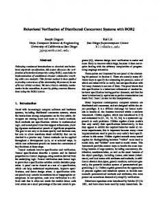
This device is an adapter which wraps around the actual piece of hardware, the ADCS Mainpanel, and connects it to the simulation. The Panel Emulator is equipped with the same microcontrollers as the Sidepanels. They are used to emulate the five Sidepanels which would normally talk to the Mainpanel. But instead of reading sensor data, the Sidepanels exchange data with a Beaglebone that in turn gets its data from the simulation. All programmable devices are shown in the block diagram Fig. 7–17.

Fig. 7–17: Block diagram of the Panel Emulator

7.3.1

Board Layout

The Panel Emulator consists of a Beaglebone and five microcontrollers. Its PCB shown in Fig. 7–18 and appendix A.5 has four identical areas for every Sidepanel and an area for the Toppanel that omits the usual Picolock-12 socket because the Toppanel connects over PC/104 to the Mainpanel. The Beaglebone is attached upside-down with pin headers [19, 20]. The PC/104 connects to the Mainpanel and to the FakeCDH board which emulates the functionality of MOVE-II's CDH and EPS. The schematics of the Panel Emulator are given in Appendix 1.

Page 32

HiL Environment

Fig. 7–18: Rendering of the Top of the Panel Emulator PCB

7.3.2

Data Flow

The block diagram Fig. 7–19 shows all major data flows of the complete HiL environment including those within the Panel emulator. The single board computer (SBC) Beaglebone Black Wireless connects over ethernet or WiFi to the simulation PC and transfers data over a TCP connection using the WebSockets protocol. It relays that data to the Sidepanel microcontrollers over SPI. The rate of this communication is set by the simulation to 10 Hz. Every transfer over WebSockets or SPI includes sending data from the simulation towards the Mainpanel, e.g. simulated sensor readings, and receiving data from the Mainpanel, e.g. desired magnetorquer currents. The Mainpanel talks to the Sidepanel microcontrollers on the Panel emulator in the same way as it would to the real Sidepanels. It requests a data structure at a modespecific update frequency over SPI and writes back another data structure containing the magnetorquer commands. This transfer utilizes the direct memory access (DMA) capabilities of the Sidepanel microcontrollers.

Page 33

HiL Environment

Fig. 7–19: Block diagram of the major data flows in the HiL environment

7.3.3

Beaglebone

The Beaglebone Black Wireless was selected for its relatively high computational power, its WiFi capability, and the fact that Beaglebones already found widespread use in the MOVE-II project. Due to latency issues, this Beaglebone uses an ethernet connection over a USB adapter instead of the native WiFi interface. Connecting it over ethernet eliminates the possibility to hang the Mainpanel including the Panel Emulator from a thread and put it in a Helmholtz cage, which would result in a combination of full ADCS and controller-only approach. The Beaglebone runs the relay program Panel Emulator [17] which is written in C++ and translates from the WebSockets protocol to the SPI bus where it forwards the data from the simulation PC to the Sidepanel microcontrollers. When executing the program, the main loop (/panelEmulator/src/main.cpp, line 174) [17] asks for the IP and port of the simulation PC and then tries to open a WebSockets connection to it. Upon success, it will keep this connection open until the user presses the enter key which results in closing the connection and terminating the program. As long as the connection is open, a new message from the simulation PC will trigger execution of the function on_message (/panelEmulator/src/main.cpp, line 109) [17] which stores the content of the message from the PC and starts a for loop to process it for every Sidepanel. In the loop, the data is converted to the SidepanelData data structure that is defined in the firmware of the ADCS Mainpanel and Sidepanel (/src/api/include/Control.hpp, line 214) [12] and calls the spi_transfer function (/panelEmulator/src/main.cpp, line 35) [17]. First, the data structure data of type SidepanelData is written to the microcontroller over SPI. After that, the data structure control of type SidepanelControl (/src/api/include/Control.hpp, line 348) [12] is read back from the microcontroller and its header bytes and the checksum get verified. If one of those checks should fail, the transfer gets reattempted for a maximum of 32 times. Back in the on_message function, the control data structure is converted to the type HiL_Control_Panel. Once the for loop has completed, the HiL_Control_Panel Page 34

HiL Environment

structure gets sent over the WebSockets connection to the simulation PC and the Panel Emulator program waits for the next message from the simulation PC. The Beaglebone connects upside-down to the pin headers P8 and P9 on the Panel Emulator PCB. The push-button S1 is a power button. Pressing it will result in a proper shutdown of the Beaglebone which should avoid file system corruption that might occur when cutting the power while the Beaglebone is in the middle of a write operation. The push-button S2 selects the boot device of the Beaglebone if the user wants to boot from a micro SD card. 7.3.4

Sidepanel Microcontrollers

The Sidepanels and the Toppanel have one ATXMega64A4U-AU microcontroller each. The Mainpanel reads the data structure containing the sensor data as a DMA transfer at regular intervals. At the same time, it also writes the data structure containing the current command to the Sidepanel. The microcontrollers 1U2 to 4U2 and U3 shown in Fig 7.2 on the Panel Emulator are of the same type as those on the Sidepanels. They act as a slave to the Mainpanel and to the Beaglebone. All transfers are DMA and the data does not need to get converted between different structures, so the main.cpp of the microcontrollers (/spiSlaveBuffer/src/main.cpp) [17] does only instantiate two DMA objects which are defined in the ADCS software Repository (/src/api/lib/SPI/DMA/DmaSpiSlave.cpp) [12], (/src/api/lib/SPI/DMA/DmaSpiSlaveHil.cpp) [12]. On every transfer, the red status LED of the corresponding microcontroller is toggled.

Fig. 7–20: Rendering of the Bottom of the Panel Emulator PCB

Page 35

HiL Environment

Each microcontroller has a PDI header 1P2 to 4P2 and P3 shown in Fig 7.3 for programming and debugging output over the UART bus. One red LED 1D1 to 4D1 and D6 shows the status of the Sidepanel. The LED 1D2 to 4D2, D7 shows whether the microcontroller is held in reset over PDI. The reset LED is active low. The LED 1D3 to 4D3, D8 shows the state of the PDI data line. The LED 1D4 to 4D4, D9 shows if the Sidepanel is supplied with 5V. The LED 1D5 to 4D5, D10 shows the state of the 3.3V supply. As the Panel Emulator has its own power supply described in section 7.2.5, the microcontrollers on the Panel Emulator will not switch off when the Mainpanel cuts power to the Sidepanel 3.3V lines. 7.3.5

Additional Circuitry

The 3.3V regulator U1 shown in fig 7.3 converts from the 5V bus of the EPS to the supply voltage of the microcontrollers. The Panel Emulator is designed to be supplied by the FakeCDH board which does not supply enough current on the 3.3V bus. Three UART buses from the Beaglebone are routed to the pin headers UART1, UART4, UART5. They allow to read the serial debug output from the panel microcontrollers when connecting a UART header to the PDI header of the microcontroller. The pin header I2C allows access to the I²C bus of the Beaglebone if needed. The LEDs D11 and D12 indicate that the 5V and the 3.3V line on the Panel Emulator have power. The switch SW1 cuts the 5V line to the regulator U1 and the Beaglebone, thereby switching the Panel Emulator off.

7.4

HiL Stack

The ADCS Mainpanel, the Panel Emulator, and the FakeCDH form the HiL Stack depicted in Fig. 7–22 and Fig. 7–21. The Panel Emulator connects over four Picolock cables and the PC/104 stack to the Mainpanel. The FakeCDH acts as the CDH and commands the Mainpanel over the respective SPI bus. The FakeCDH connects over WiFi to the university network, the Panel Emulator connects over Ethernet to the university network to minimize the roundtrip time between simulation and hardware.

Fig. 7–21: Block Diagram of HiL Stack

Page 36

HiL Environment

Fig. 7–22: HiL Stack with Power Supply Connected

Page 37

Controller Modes

8

Controller Modes

The ADCS shall point the satellite to the sun to increase the generated solar power and to allow operation of the solar cell characterization payload. To reduce the tumbling rate after separation from the CubeSat deployer, a detumbling controller will be used too. The ADCS team has developed two different detumbling strategies and two different sunpointing strategies. All four, and additionally a blended strategy using detumbling and sunpointing alternatively, shall be investigated. This chapter will describe all controllers and specify the test runs of the HiL environment for every controller. The orbital parameters for the circular 575 km sun-synchronous orbit of MOVE-II are given in the appendix Tab. A 4. The environmental parameters for realistic worst-case environmental conditions and the sensor model characteristics are given in the appendix Tab. A 5. Some testcases use ideal conditions where the disturbances, the sensor noise and bias, and the current threshold of the magnetorquers are turned off. The Mainpanel configuration can be found in appendix Tab. A 6. They allow to switch between B-dot detumbling and the sunpointing controller. Additionally, the gain matrix, the magnetorquer configuration, the primary sensor, the spin rate, and the behavior during eclipse can be set.

8.1

B-Dot Detumbling

The simplest controller for detumbling a satellite using magnetorquers is the B-dot controller. Its control law presented in Eq. ( 8-1 ) is a proportional relationship between 𝑏𝑜𝑑𝑦

the derivative of Earth’s magnetic field vector in satellite body frame 𝐵̇𝐸𝑎𝑟𝑡ℎ and the desired magnetic control moment. The variable k is the gain of the B-dot controller. 𝑏𝑜𝑑𝑦 𝑚𝑐𝑜𝑛𝑡𝑟𝑜𝑙 = 𝑘𝐵̇𝐸𝑎𝑟𝑡ℎ

Eq. ( 8-1 )

The magnetic dipole moment mcontrol does not affect the angular velocity of the satellite directly. The magnetic dipole moment of the satellite, which might include a parasitic dipole due to ferromagnetic materials inside the satellite, interacts with Earth’s magnetic field. This interaction causes a torque affecting the satellite as stated in Eq. ( 8-2 ). 𝑏𝑜𝑑𝑦

𝜏𝑚𝑎𝑔𝑛𝑒𝑡𝑖𝑐 = (𝑚𝑐𝑜𝑛𝑡𝑟𝑜𝑙 + 𝑚𝑝𝑎𝑟𝑎𝑠𝑖𝑡𝑖𝑐 ) × 𝐵𝐸𝑎𝑟𝑡ℎ

Eq. ( 8-2 )

The usage of the magnetic field’s derivative ensures that the magnetic dipole moment vector will always result in a torque vector that reduces the angular velocity. A detailed derivation can be found in [21]. 8.1.1

Testcases

The two testcases aimed at characterizing the B-dot controller’s performance are given in Tab. 8–1. The maximum tumbling rate expected after deployment from an ISIS deployer [22] is estimated to be smaller than 0.2 rad/s in every axis. To verify that the detumbling controller can recover from angular velocities at this order of magnitude, the initial tumbling rate will be set to 0=(0.5 0.5 0.5) rad/s. Another test with an initial tumbling rate of 0=(0.1 0.1 0.1) rad/s will be performed to evaluate the performance when switching from sunpointing mode to detumbling. Page 38

Controller Modes

Tab. 8–1: B-Dot Detumbling Testcases Controller

Conditions

Initial Velocity [rad/s]

Description

1

B-Dot Detumbling

Realistic

(0.5 0.5 0.5)

Detumbling run, Gain 100000

2

2

B-Dot Detumbling

Realistic

(0.1 0.1 0.1)


2

#

8.2

Runtime [orbits]

Non-Spinning Sunpointing Controller

Sunpointing utilizes a 5-dimensional state-feedback controller. The gain matrix is found by a linear-quadratic regulator (LQR) algorithm. The design of this controller is detailed in [6], where it is referred to as reduced-axis control. The state vector shown in Eq. ( 8-3 ) consists of the X- and Y-component of the sun vector SECI and all three components of the gyroscope measurement body. All 5 variables shall be minimized by the controller.

𝑥 = (𝑆𝐸𝐶𝐼,𝑥

𝑆𝐸𝐶𝐼,𝑦

𝑏𝑜𝑑𝑦

𝑏𝑜𝑑𝑦

𝜔𝑥

𝜔𝑦

𝑏𝑜𝑑𝑦

𝜔𝑧

)′

Eq. ( 8-3 )

The state-feedback controller calculates the desired control torque u, which is necessary for achieving sun-pointed attitude and minimizing the angular velocity. The control torque is 3-dimensional, and the state vector is 5-dimensional, so the gain matrix KRED has 5x3 components. The control law is noted in Eq. ( 8-4 ) [24].

𝑢 = −𝐾𝑅𝐸𝐷 𝑥

Eq. ( 8-4 )

0.0321 0.0005 0.0543 −4.2636 0.0648 𝐾𝑅𝐸𝐷 = (−0.0521 −0.0005 0.0678 −3.6578 0.1582 ) −0.0158 0.0032 −0.1848 −0.8293 −0.5196 The controller cannot stabilize the satellite if the parasitic dipole is estimated at worstcase level. A more aggressive gain matrix KRED,multiplied was found heuristically that can compensate the disturbance torque of the parasitic dipole [6]. −0.0000 0.7606 −92.7963 −0.0000 0.0000 𝐾𝑅𝐸𝐷,𝑚𝑢𝑙𝑡𝑖𝑝𝑙𝑖𝑒𝑑 = (−0.7606 0.0000 −0.0000 −74.7403 −0.0335) 0.0067 0.0000 −0.0000 0.0590 −0.3803 According to Eq. ( 7-3 ), the control torque acting on the satellite is the cross-product of the magnetic dipole moment vector generated by the magnetorquers and the magnetic field of the Earth. A mapping function shown in Eq. ( 8-5 ) determines a suitable dipole moment vector to obtain the desired torque vector. 𝑏𝑜𝑑𝑦

𝑚𝑐𝑜𝑛𝑡𝑟𝑜𝑙 =

𝑢 × 𝐵𝐸𝑎𝑟𝑡ℎ 𝑏𝑜𝑑𝑦

‖𝐵𝐸𝑎𝑟𝑡ℎ ‖

Eq. ( 8-5 )

The control torque u and Earth’s magnetic field must be perpendicular for Eq. ( 8-5 ) to be true. The part of u parallel to the magnetic field is lost in this equation. This is a common limitation of magnetic attitude control. The spacecraft is only controllable in the plane perpendicular to the magnetic field [23]. When in sunpointed attitude, the magnetic field will perform one revolution around the satellite per orbit, so a single axis will stay uncontrollable for a few minutes every orbit. Any disturbance torque affecting Page 39

Controller Modes

an uncontrollable axis will increase the pointing error until it has rotated the spacecraft in an attitude which allows the satellite to counteract the disturbance. Such events will lead to pointing errors larger than 45° and can result in instability of the sunpointing controller. 8.2.1

Testcases

Preliminary analysis has shown that the non-spinning sunpointing controller’s performance is better with low initial angular velocities. Therefore, testcases 3 and 5 shown in Tab. 8–2 will set the initial angular velocity to 0=(0.01 0.01 0.01) rad/s which translates to 1°/s and is the minimum velocity that the B-dot controller can achieve. Testcases 4 and 6 will set the initial angular velocity to 0=(0.1 0.1 0.1) rad/s which is the estimated angular velocity after separation from the launcher and therefore a reasonable worst-case estimate for the sunpointing controller. Testcases 3 and 4 assume ideal conditions, i.e. no disturbances or sensor inaccuracies, while the realistic conditions in testcase 5 and 6 set the disturbances, sensor noise, and sensor bias to worst-case levels. Tab. 8–2: Non-Spinning Sunpointing Controller Testcases # 3

4

5

6

8.3

Controller Non-Spinning Sunpointing Controller Non-Spinning Sunpointing Controller Non-Spinning Sunpointing Controller Non-Spinning Sunpointing Controller

Conditions


Ideal

(0.01 0.01 0.01) Gain KRED,multiplied

4

Ideal

(0.1 0.1 0.1)

Gain KRED,multiplied

4

Realistic


6

Realistic

(0.1 0.1 0.1)

6

Description


Runtime [orbits]

Detumbling Sunpointing Controller

When setting the first two columns of the gain matrix to zero, the sun vector will not affect the torque command anymore. The remaining coefficients will result in a controller that only minimizes the angular velocity measured by the gyroscope. A gain matrix that is useful for detumbling is given in Eq. ( 8-6 ) 0 0 −10 1 1 𝐾𝑑𝑒𝑡𝑢𝑚𝑏𝑙𝑖𝑛𝑔 = (0 Eq. ( 8-6 ) 0 1 −10 1 ) 0 0 1 1 −10 The non-diagonal terms mitigate an alignment of the commanded torque vector and the magnetic field which would result in uncontrollability of the satellite. Due to the mapping function of the sunpointing controller shown in Eq. ( 8-5 ), no magnetic dipole moments parallel to the magnetic field can be commanded which should make this controller more power-efficient than the B-dot detumbling controller discussed in section 8.1. Page 40

Controller Modes

8.3.1

Testcases

The detumbling sunpointing controller faces the same conditions as the B-dot controller. In testcase 7, the initial angular velocity is 0=(0.5 0.5 0.5) rad/s, which is identical to testcase 1. The initial velocity of testcase 8 is 0=(0.1 0.1 0.1) rad/s and identical to testcase 2, only the runtime decreases because of the expected faster detumbling. Testcase 7 and 8 are stated in Tab. 8–3. Tab. 8–3: Detumbling Sunpointing Controller Testcases #

Controller Detumbling 7 Sunpointing Controller Detumbling 8 Sunpointing Controller

8.4

Conditions


Description

Runtime [orbits]

Realistic

(0.5 0.5 0.5)

Gain KDetumbling

2

Realistic

(0.1 0.1 0.1)

Gain KDetumbling

1

Gain Switching Sunpointing Controller

If the sunpointing controller becomes unstable, it needs to be reset. The angular momentum of the satellite needs to be reduced before the sunpointing controller becomes active again. A mode switcher will transition from sunpointing described in section 8.2 to the detumbling mode of the sunpointing controller described in section 8.3. Both controllers only differ in terms of their gain matrix. Updating the gain of the sunpointing controller during simulation time suffices to switch between sunpointing and detumbling mode. The criterion for switching is the angular velocity measured by the gyroscope. When exceeding the norm of the angular velocity exceeds 0.2 rad/s, the mode switcher will set the sunpointing controller to detumbling mode. After the norm falls below 0.03 rad/s, the mode switcher sets the controller to sunpointing mode again. 8.4.1

Testcases

Testcase 9 in Tab. 8–4 executes the gain switching sunpointing controller at realistic conditions and a high initial velocity of 0=(0.1 0.1 0.1) rad/s so the performance can be compared to that of the non-spinning sunpointing controller in testcase 6. Tab. 8–4: Gain Switching Sunpointing Controller Testcase #

Controller Gain Switching 9 Sunpointing Controller

Conditions


Description

Realistic

(0.1 0.1 0.1)

Switch between KDetumbling and KRED,multiplied based on the angular velocity

Runtime [orbits] 4

Page 41

Controller Modes

8.5

Spinning Sunpointing Controller

A modification of the state-feedback controller discussed in section 8.2 sets the desired angular velocity as in Eq. ( 8-7 ) to command a spin around the z axis of the satellite. 0 𝜔𝑠𝑝𝑖𝑛 = ( 0 ) [𝑟𝑎𝑑/𝑠] Eq. ( 8-7 ) 0.1 The controller uses a different gain matrix derived via the LQR algorithm shown in Eq. ( 8-8 ) [24].

𝑢 = −𝐾𝑆𝑃𝐼𝑁 𝑥

Eq. ( 8-8 )

0.0321 0.0005 0.0543 −4.2636 0.0648 𝐾𝑆𝑃𝐼𝑁 = (−0.0521 −0.0005 0.0678 −3.6578 0.1582 ) −0.0158 0.0032 −0.1848 −0.8293 −0.5196 Like the non-spinning sunpointing controller, the gain matrix needed manual adjustments for compensating the disturbances of the parasitic dipole. The resulting gain matrix KSPIN,multiplied will be used for all simulation runs of the spinning sunpointing controller. 0.0680 0 −20.0000 −1.0340 0.0050 𝐾𝑆𝑃𝐼𝑁,𝑚𝑢𝑙𝑡𝑖𝑝𝑙𝑖𝑒𝑑 = ( 0 −0.0620 −1.4360 −20.0000 0.0040 ) 0 0 0.0008 0.0004 −3.4000 The major advantage of a spin controller is that no axis will stay uncontrollable for a long time. The non-spinning controller will experience one revolution of the magnetic field every orbit. An axis can stay uncontrollable for several minutes. The spinning controller will experience one revolution of the magnetic field every minute. A single axis will stay uncontrollable for just a few seconds. Due to the high spin rate and to the angular momentum, any disturbance torques are less likely to affect the pointing error of the spinning sunpointing controller as much as with the non-spinning controller. MOVE-II is not particularly suitable for spin control, because it does not have its principal axis of inertia aligned with the Z-axis that shall be directed towards the sun. A rotation around the Z-axis without an active controller will immediately result in precession of the angular rotation vector. The spin controller always needs to counteract the precession of the spin axis, even during eclipse. This additional torque results in an additional electrical power draw. The inertia tensor of MOVE-II is stated in section 7.1.3.1. 8.5.1

Testcases

As shown in Tab. 8–5, the spinning sunpointing controller will be run in an ideal environment in testcase 10. The simulation parameters will be the same as in testcase 4. Testcase 11 runs the spinning controller at realistic conditions identical to testcase 6. Since the spinning controller copes well with high initial velocity, testcases with a reduced initial angular velocity have been omitted. Testcase 11 will be the reference for the repeat accuracy analysis and for the sensitivity analysis.

Page 42

Controller Modes

Tab. 8–5: Spinning Sunpointing Controller Testcases #

Controller

Spinning 10 Sunpointing Controller Spinning 11 Sunpointing Controller Detumbling, Spinning 12 Sunpointing Controller

Conditions


Description

Ideal

(0.1 0.1 0.1)

Gain KSPIN,multiplied, Spin rate 0.1 rad/s

4

Realistic

(0.1 0.1 0.1)


4

(0.1 0.1 0.1)

Detumble to 0.131 rad/s, then switch to Sunpointing, Gain KSPIN,multiplied, Spin rate 0.1 rad/s, Start briefly before eclipse.

4

Realistic

Runtime [orbits]

To find out by how much the jitter introduced by the asynchronous devices like the simulation PC and the Beaglebone on the Panel Emulator affects the results of the HiL simulation, testcase 11 is repeated two times. Testcase 13 stated in Tab. 8–6 will give an indication of the typical error of the HiL setup during the second orbit. This error should be kept in mind while analyzing the performance differences that the sensitivity analysis will yield. Testcase 14 runs the spinning controller for over 24 hours and shall verify its stability for long durations. Tab. 8–6: Spinning Sunpointing Controller Testcases for Repeat Accuracy Analysis #

Controller

Spinning 13 Sunpointing Controller Spinning 14 Sunpointing Controller

8.6

Conditions


Description

Realistic

(0.1 0.1 0.1)

Repetition of testcase 11, Gain KSPIN,multiplied, Spin rate 0.1 rad/s

Realistic

(0.1 0.1 0.1)

Investigate long-term stability, Gain KSPIN,multiplied, Spin rate 0.1 rad/s

Runtime [orbits] 2

16

Sensitivity Analysis

Based on the run specified in testcase 11, the sensitivity of the controller to inaccuracies in the simulation model shall be observed with a series of tests. Every test will change one quantity in the model, e.g. the noise level of the magnetometer, or the initial velocity. Investigating the behavior of the spinning sunpointing controller for a broad variety of parameter sets will give an indication, if the controller is particularly sensitive to one dimension of the parameter space. The performance of the controller in those testcases is quantified by comparing the mean pointing error and the generated battery charge per orbit. When calculating these performance measures, the first orbit of every run is ignored to give the controller the time necessary for attaining sunpointed attitude. 8.6.1

Testcases

All testcases stated in Tab. 8–7 are identical to testcase 11 except for their runtime and one or more modified parameters stated in the description field of the table. Page 43

Controller Modes

Tab. 8–7: Spinning Sunpointing Controller Testcases for Sensitivity Analysis #

Controller

Spinning 15 Sunpointing Controller Spinning 16 Sunpointing Controller Spinning 17 Sunpointing Controller Spinning 18 Sunpointing Controller Spinning 19 Sunpointing Controller Spinning 20 Sunpointing Controller Spinning 21 Sunpointing Controller Spinning 22 Sunpointing Controller Spinning 23 Sunpointing Controller Spinning 24 Sunpointing Controller Spinning 25 Sunpointing Controller Spinning 26 Sunpointing Controller Spinning 27 Sunpointing Controller Spinning 28 Sunpointing Controller Spinning 29 Sunpointing Controller Spinning 30 Sunpointing Controller Spinning 31 Sunpointing Controller

Conditions


Description

Runtime [orbits]

Realistic

(0.1 0.1 0.1)

2x Magnetic Disturbance, 2x Gravity Gradient, 10x Higher Air Density, Gain KSPIN,multiplied, Spin rate 0.1 rad/s,

2

Realistic

(0.1 0.1 0.1)

0.5x Disturbances, Gain KSPIN,multiplied, Spin rate 0.1 rad/s

2

Realistic

(0.1 0.1 0.1)

2x Magnetometer noise, Gain KSPIN,multiplied, Spin rate 0.1 rad/s

2

Realistic

(0.1 0.1 0.1)

2x Gyroscope noise, Gain KSPIN,multiplied, Spin rate 0.1 rad/s

2

Realistic

(0.1 0.1 0.1)

2x Sun sensor noise, Gain KSPIN,multiplied, Spin rate 0.1 rad/s

2

Realistic

(0.1 0.1 0.1)

2x Magnetometer bias, Gain KSPIN,multiplied, Spin rate 0.1 rad/s

2

Realistic

(0.1 0.1 0.1)

2x Gyroscope bias, Gain KSPIN,multiplied, Spin rate 0.1 rad/s

2

Realistic

(0.1 0.1 0.1)

Sun sensor bias of 10°, Gain KSPIN,multiplied, Spin rate 0.1 rad/s

2

Realistic

(0.1 0.1 0.1)

Sun sensor field-of-view reduced to 100 degrees, Gain KSPIN,multiplied, Spin rate 0.1 rad/s

2

Realistic

(0.1 0.1 0.1)

Coil driver does not ignore currents, Gain KSPIN,multiplied, Spin rate 0.1 rad/s

2

Realistic

(0.1 0.1 0.1)

Coil driver ignores currents below 100 mA, Gain KSPIN,multiplied, Spin rate 0.1 rad/s

2

Realistic

(0.1 0.1 0.1)

5x Sample time for dynamics model, Gain KSPIN,multiplied, Spin rate 0.1 rad/s

2

Realistic

(0 0 0)

Zero initial angular velocity, Gain KSPIN,multiplied, Spin rate 0.1 rad/s

2

Realistic

(0.5 0.5 0.5)

5x Initial angular velocity, Gain KSPIN,multiplied, Spin rate 0.1 rad/s

2

Realistic

(0.1 0.1 0.1)

Start time shifted to eclipse, Gain KSPIN,multiplied, Spin rate 0.1 rad/s

2

Realistic

(0.1 0.1 0.1)

Lower orbit of 545x555 km, Gain KSPIN,multiplied, Spin rate 0.1 rad/s

2

Realistic

(0.1 0.1 0.1)

Diagonal inertia tensor, Gain KSPIN,multiplied, Spin rate 0.1 rad/s

2

Page 44

Controller Modes

8.7

No Controller

The simulation model includes a power estimator that calculates the power generated by the solar cells and subtracts the power consumption of the ADCS and the remaining subsystems to obtain the power that is charged into the battery. The power estimator can give a prediction if the satellite stays power-positive during the simulation run. All testcases assume that the satellite runs in nominal mode except for testcase 32, which simulates a tumbling satellite in safe mode. Several events can cause the satellite to enter safe mode and switch off the ADCS which leaves the satellite tumbling freely. Safe mode is activated if the temperature of one subsystem rises above a critical threshold or the battery’s state-of-charge (SoC) falls below 10%. If the satellite does not achieve more than 10 min uptime on three consecutive boots, it transitions to a special safe mode called RawResQ which allows for recovering from a corruption of the nominal operating system. In safe mode, the satellite consumes 1.88 W continuously, which is a very high power consumption for the safe mode of a 1-unit CubeSat. A breakdown of the power consumptions is given in Tab. 8–8. Tab. 8–8: Power Consumption of the Subsystems Active in Safe Mode System

Power Consumption

EPS

0.65 W

COM

1.00 W

CDH

0.23 W

Total

1.88 W

If too much energy is drained from the batteries, the under-voltage protection (UVP) circuit of the EPS modelled in 7.1.5.3 will shut down the satellite. The power consumption reduces to 0.008 W during UVP shutdown which allows the batteries to recharge and end the UVP condition. 8.7.1

Testcases

The simulation parameters for testcase 32 in Tab. 8–9 are similar to the previous ones except the gain matrix is filled with zeros to ignore the controller commands. Tab. 8–9: Tumbling Testcase for Analyzing Behavior during Safe Mode #

32

Controller

No Controller

Conditions


Realistic

Verify power budget of safe mode (1.88W) when tumbling, (0.01 0.01 0.01) Under-voltage protection switches the satellite off when the battery is empty

Description

Runtime [orbits]

8

Page 45

Test Results

9

Test Results

After executing all runs described in chapter 8, the results will be analyzed and discussed in this chapter. The order of the subsections will be the same as in the previous chapter. The performance of the detumbling controllers is quantified with the time it takes until the target velocities 0.131 rad/s and 0.017 rad/s. Additionally, the energy drained from the batteries until reaching the target velocity is stated. The energy estimation includes the power generated by the solar panels, the ADCS’ power consumption, and an estimate of the rest of the satellite’s power consumption in nominal mode. The eclipse period is visualized with a grey background in the result graphs. The performance of the sunpointing controllers is quantified with the mean pointing error and the amount of energy charged in to the battery per orbit. Again, the battery power is the difference between the solar power and the sum of ADCS and remaining subsystems power in nominal mode. The first orbit is not considered to give the controller some time for alignment and stabilization.

9.1

B-Dot Detumbling

The detumbling controller reliably reduces the angular velocity of the satellite to less than 0.02 rad/s. The ADCS will send the DETUMB: REACHED signal to the state machine of the CDH when the angular velocity is lower than the detumbling threshold. The threshold is set to 0.017 rad/s for an ADCS configuration, where the non-spinning sunpointing controller is the default. For the more robust spinning sunpointing controller, the threshold will be set to 0.131 rad/s.

Fig. 9–1: Testcase 1, Detumbling from 0.87 rad/s to 0.017 rad/s

Page 46

Test Results

Fig. 9–1 and Fig. 9–2 show the B-Dot Detumbling Controller detumbling until the DETUMB: REACHED signal is sent with the lower threshold of 0.017 rad/s configured. The minimum velocity achieved is 0.011 rad/s. The detumbling time and energy consumption of the whole satellite during detumbling for both thresholds is listed in Tab. 9–1. The energy consumption is measured at the battery, so it includes the estimated power consumption of the ADCS, the remaining systems in nominal mode, and the power generation from the solar cells.

Fig. 9–2: Testcase 2, Detumbling from 0.173 rad/s to 0.017 rad/s

Fig. 9–1 and Fig. 9–2 show that the B-dot detumbling controller affects all axes almost equally, especially for Testcase 1. The initial angular velocity vector is not aligned with the principal axis of inertia of the satellite. Therefore, a gyroscopic moment causes the angular velocity vector to precede in a periodic movement. The corresponding rigidbody equation is explained in section 7.1.3.1. Tab. 9–1: Performance of B-Dot Detumbling Controller in Testcase 1 and 2

Time for detumbling to 0.131 rad/s

Consumed energy for detumbling to 0.131 rad/s



Testcase 1

90 min

3.5 Wh

162 min

5.8 Wh

Testcase 2

12 min

0.3 Wh

92 min

3.4 Wh

The detailed workings of the detumbling algorithm can be seen in Fig. 9–3. This figure shows a two-minute-long excerpt from Testcase 1. The uppermost plot shows the Bdot signal in body frame. The second plot shows the control dipole moment. It consists of 300ms pulses every second to allow for magnetometer measurements in-between. The third plot shows the angular velocity of the satellite. Page 47

Test Results

B-dot is obtained by computing the derivative of the magnetic field in body frame. The simple differentiation introduces considerable noise although this signal was not passed through a sensor model beforehand.

Fig. 9–3: Detailed Look at the B-Dot Detumbling Controller over Six Revolutions.

One can observe the B-dot control law described in Eq. ( 8-1 ) when comparing one component of B-dot with one component of mcontrol. They are the exact opposite with a factor of 100,000 between them, which is the gain factor used during B-dot detumbling. The maximum current is limited to 300 mA, so the maximum mcontrol is 0.091 Am² for a Sidepanel or Toppanel according to Tab. 5–3.

9.2

Non-Spinning Sunpointing Controller

The non-spinning variant was originally supposed to serve as the default sunpointing controller due to the inertia tensor of the satellite, which is not suitable for a spinning controller. The simulations performed in [6] showed stable behavior in ideal conditions. Tab. 9–2: Performance of the Non-Spinning Sunpointing Controller in Ideal Conditions Mean Pointing Error

Standard Deviation of the Pointing Error

Generated Energy per Orbit

Testcase 3

0.3°

0.42°

1.235 Wh

Testcase 4

0.37°

0.55°

1.234 Wh

Testcase 3 and 4 put the controller in an ideal environment without any disturbances or sensor noise. The initial angular velocity for testcase 3 is 0=(0.01 0.01 0.01) rad/s, the initial velocity for testcase 4 is 0=(0.1 0.1 0.1) rad/s. Both testcases show stable behavior and only a small pointing error. The power budget is positive by a wide margin because of the near-perfect attitude and the low control currents. The results of testcase 3 and 4 can be found in Tab. 9–2, the graph for testcase 4 is shown in Fig. 9–4, the graph for testcase 3 is included in the accompanying files. Page 48

Test Results

Fig. 9–4: Testcase 4, Non-Spinning Sunpointing at High Initial Velocity in Ideal Conditions.

Testcase 5 and 6 include disturbances and imperfections in the sensor models which decrease the controller’s performance. In these conditions, the non-spinning sunpointing controller shows instabilities every few orbits. This behavior shows up during long simulation runs with more than three orbits or during runs with a high initial velocity. Testcase 5 starts at a low initial angular velocity of 0=(0.01 0.01 0.01) rad/s, testcase 6 starts at a high initial velocity of 0=(0.1 0.1 0.1) rad/s. Both testcases show severe instabilities, which significantly impede the performance characteristics shown in Tab. 9–3. Tab. 9–3: Performance of the Non-Spinning Sunpointing Controller in Realistic Conditions Mean Pointing Error



Testcase 5

17.59°

24.55°

0.189 Wh

Testcase 6

30.64°

31.18°

-0.593 Wh

Page 49

Test Results

Testcase 5 shows problematic behavior at the end of every eclipse which results in a spin-up of the z axis to 0.2 rad/s and slows maneuvering to sunpointed attitude. Still, the power budget remains positive. The graph for testcase 5 can be found in the accompanying files. The behavior of testcase 6 is shown in Fig. 9–5 and shows even worse instabilities than testcase 5 in the orbits 2, 5, and 6. The power budget is negative. The only difference in the parameters of testcase 5 and 6 is the initial angular velocity. The results lead to the conclusion that the non-spinning sunpointing controller is impaired by a high angular momentum of the satellite and cannot reduce the momentum in a sustainable way. Testcase 9 covers the gain switching sunpointing controller which shall address this insufficiency of the sunpointing controller.

Fig. 9–5: Testcase 6, Non-Spinning Sunpointing at High Initial Velocity in Realistic Conditions

Page 50

Test Results

9.2.1

Uncontrollability

The instabilities of the non-spinning sunpointing controller can be attributed to the satellite lining up its desired torque vector u with the surrounding magnetic field Bbody. Section 8.2 already stated that an ADCS solely relying on magnetorquers suffers from uncontrollability in the axis parallel to the magnetic field. Fig. 9–6 shows the fifth orbit of testcase 6. Looking at the pointing error graph, one can see that it starts to increase at t=4.95 and at t=5.43 orbits. These two points in time are marked with dashed lines. The angular velocity graph shows the satellite spinning at a high rate around the z axis. Eventually the x and y velocity are also affected through the gyroscopic moments caused by the non-diagonal inertia tensor and the satellite starts tumbling. Out of this tumbling motion, it can finally stabilize itself again until experiencing the next instability.

Fig. 9–6: Detailed View on the Fifth Orbit of Testcase 6 Focusing on Instabilities

The two lower graphs show Earth’s magnetic field in body frame and the dot product of the desired torque vector u with the magnetic field Bb. The desired torque is not available directly from the Mainpanel, so it is retrieved from the Simulink controller that is executed in parallel to the Mainpanel. Page 51

Test Results

Eq. ( 7-3 ) from section 7.1.1 and Eq. ( 8-5 ) from section 8.2 define how the satellite can only exert a torque in the plane normal to the magnetic field and therefore ignores the part of the desired torque u that is parallel to the magnetic field vector. The dot product displayed in Fig. 9–6 quantifies the parallelism of u and Bb. If the dot product reaches 1 or -1, the satellite cannot generate any of the desired torque. During the instable phases, the z component of Bb is close to zero while the x and y components are relatively high. This constellation of Bb does not allow for significant torque around the x and y axes but greatly amplifies actuation around the z axis. The result is a satellite which strongly desires to correct the x and y axis and inadvertently begins to spin up the z axis until the gyroscopic moments make the satellite drift out of its uncontrollable attitude. The gain matrix favors the x and y axis because the z axis rotation does not alter the solar power production. Furthermore, the matrix has non-diagonal terms in the third row which cause a desired torque around the z axis because of the x and y error. These two characteristics of the gain matrix cause the controller to not reduce the z velocity in case of increasing x and y errors. One intuitive solution to this problematic behavior would be to increase the z axis gain and eliminate the non-diagonal terms. Implementing a completely diagonal gain matrix resulted in even longer instabilities though. The satellite stays trapped in the noncontrollable attitude because every drift out of this attitude allows for small x or y axis torque which moves the satellite back in the non-controllable attitude. The solution to the uncontrollable behavior is a rotation that changes the magnetic field vector periodically. Wisniewski [23] designed an attitude control system for a gravity gradient-stabilized satellite that changed its orientation towards the magnetic field by 90° for every fourth of an orbit as shown in Fig. 9–7. MOVE-II is not gravity gradientstabilized and needs a switch of the controllable axes more often than once every quarter orbit, so a non-spinning controller seems to be inadequate for this ADCS.

Fig. 9–7: Controllable Axes of a Gravity Gradient-Stabilized Satellite with Magnetorquers [23]

Page 52

Test Results

9.3

Detumbling Sunpointing Controller

The gyroscope signal is less noisy than the B-dot signal. Also, the sunpointing controller with the mapping function, showed more dynamic behavior than the B-dot detumbling controller. These two characteristics make the detumbling sunpointing controller faster and more accurate than the B-dot sunpointing controller. When detumbling from the same two initial velocities as the B-dot controller, the detumbling sunpointing controller is indeed faster. The norm of the minimum velocity achieved is 0.006 rad/s while the B-dot controller could only reduce the velocity to 0.011 rad/s.

Fig. 9–8: Testcase 7, Detumbling with Sunpointing Controller from 0=(0.5 0.5 0.5) rad/s

Testcase 7 and 8 specified in 8.3.1 define detumbling runs from 0=(0.5 0.5 0.5) rad/s and 0=(0.1 0.1 0.1) rad/s. The performance characteristics are shown in Tab. 9–4, show graphs of the two detumbling runs. Tab. 9–4: Performance of Detumbling Sunpointing Controller in Testcase 7 and 8





Testcase 7

25.7 min

1.25 Wh

43.5 min

1.55 Wh

Testcase 8

1 min

0.06 Wh

5.3 min

0.21 Wh

The detumbling is about 3x faster compared to B-dot. After detumbling, the controller experiences upsets, which increase the angular velocity again. This unstable behavior could not be observed with the B-dot detumbling controller which led to the decision to keep B-dot as the default detumbling controller on the mission. Page 53

Test Results

Fig. 9–9: Testcase 8, Detumbling with Sunpointing Controller from 0=(0.1 0.1 0.1) rad/s

Similar to the non-spinning sunpointing controller, the instabilities correlate with an alignment of the desired torque vector u and the magnetic field vector Bbody. Fig. 9–10 gives the dot product of these quantities which is near 1 or -1 almost all the time, indicating an uncontrollability.

Fig. 9–10: Testcase 8, Dot Product of Desired Torque and Magnetic Field Vector

9.4

Gain Switching Sunpointing Controller

The combination of non-spinning and detumbling sunpointing controller was expected to limit the angular momentum in case of instable behavior of the non-spinning sunpointing controller. Testcase 9 described in section 8.4.1 describes the parameters, when the gain of the sunpointing controller switches to detumbling behavior. Fig. 9–11 shows the behavior of this hybrid controller. To reduce the initial velocity, the detumbling gain matrix is used. Detumbling takes over 20 minutes although the same Page 54

Test Results

initial velocity was removed from the satellite in just 4 minutes during Testcase 8. This massive difference can be attributed to the uncontrollability issue described in 9.2.1, to which every non-spinning control algorithm is susceptible. After switching to the sunpointing gain matrix, the satellite reduces the pointing error to 50° and becomes unstable shortly after that. This causes the mode switcher to activate the detumbling gain matrix again. After exiting the first eclipse, the detumbling is completed in a few minutes and the sunpointing mode succeeds in pointing the satellite to the sun with less than 20° of error for the following 3 orbits.

Fig. 9–11: Testcase 9: Switching between Detumbling and Non-Spinning Sunpointing Controller

The overall performance of the gain switching controller stated in Tab. 9–5 is not superior to that of the non-spinning sunpointing controller. Instead of a solution to the occasional instabilities of the non-spinning sunpointing controller, the gain-switching controller is just a combination of two controllers which tend to end up in an uncontrollable attitude. Replacing the detumbling sunpointing controller with the B-dot controller would be a viable method to reliably reset the non-spinning sunpointing Page 55

Test Results

controller after showing instable behavior. But the low speed of B-dot would make the detumbling phases longer and therefore impede the power budget more than the instabilities of the non-spinning sunpointing controller. Tab. 9–5: Performance of the Gain Switching Controller in Realistic Conditions

9.5

Mean Pointing Error



17.47°

18.63°

0.269 Wh

Spinning Sunpointing Controller

The non-spinning sunpointing controllers exhibit unstable behavior whenever the axis, which is aligned with the magnetic field and thus is uncontrollable, experiences a high disturbance torque. The natural solution to this problem is a spinning satellite because any axis can only become uncontrollable for a short time then [25].

Fig. 9–12: Testcase 10, Spinning Sunpointing in Ideal Conditions

Page 56

Test Results

As MOVE-II was built with a non-spinning sunpointing controller in mind, the inertia tensor’s principal axis does not align with the spin axis. The spin will cause a gyroscopic moment that needs to be compensated [26]. Testcase 10 shown in Fig. 9–12 puts the spinning sunpointing controller in an ideal environment. For the first few minutes the controller reduces the velocity of the x- and y-axis and stabilizes the z-axis velocity at the desired spin rate of 0.1 rad/s. After that, the controller tries to point the spin axis to the sun which takes about 20 minutes. The consumed energy until getting power-positive is 0.86 Wh, which is more than the energy that the non-spinning sunpointing controller usually consumes for the same maneuver.

Fig. 9–13: Testcase 11, Spinning Sunpointing at High Initial Velocity in Realistic Conditions

Testcase 11 shown in Fig. 9–13 executes the spinning sunpointing controller in a realistic environment with all disturbances and sensor inaccuracies at worst-case level. The controller remains stable and achieves a mean pointing error of 20.66°, which suffices to keep the satellite power-positive with a surplus energy of 0.358 Wh per orbit. The alignment time reduces to 5.1 minutes until the satellite is power-positive. The Page 57

Test Results

disturbances seem to help the spinning controller with aligning itself and thus question the test approach of using worst-case disturbances to verify correct operation at smaller disturbances. The influence of the disturbance torques on the alignment time are discussed in section 9.7.2. Testcase 12 simulates the launch and early operations phase (LEOP) of the satellite. After separation from the launcher, the initial velocity is estimated at 0=(0.1 0.1 0.1) rad/s. When switching on the ADCS, the state machine HORST will command it to go B-dot detumbling first and transition to spinning sunpointing as soon as the norm of the angular velocity falls below 0.131 rad/s. The detumbling period ends after 10 minutes and the sunpointing controller shows stable behavior throughout the rest of the simulation run.

The starting time was timed so that the satellite remains not sunpointed or in eclipse for the longest probable time. This gives the maximum energy that the ADCS will draw from the battery until achieving a power-positive attitude. The amount of energy used for getting power-positive is critical after experiencing a shutdown due to a depleted battery. Section 9.7.1 discusses this issue in detail. Page 58

Test Results

The performance measures of the spinning sunpointing controller in testcase 10 to 12 are given in Tab. 9–6. Tab. 9–6: Performance of the Spinning Sunpointing Controller in Testcase 10, 11, 12

9.5.1

Mean Pointing Error



Testcase 10

1.55°

0.98°

1.034 Wh

Testcase 11

20.66°

7.73°

0.358 Wh

Testcase 12

22.03°

9.25°

0.214 Wh

Repeat Accuracy of the HiL Environment

Both the simulation PC and the Beaglebone in the Panel Emulator use operating systems with asynchronous kernels which add an unpredictable delay to the data packets they are processing. The university network that connects both may add even more jitter. A HiL run will yield different results on each execution because of these varying delays. Tab. 9–7: Performance of the Spinning Sunpointing Controller in Testcase 13 and 14 Mean Pointing Error



Testcase 13

20.38°

7.60°

0.370 Wh

Testcase 14

20.44°

7.66°

0.366 Wh

This issue was investigated with testcase 13 described in 8.5.1. This run had the same parameters as testcase 11 and gives an indication on how large the variance of simulation results because of varying delays in the test setup is. The upper row of Tab. 9–8 gives the differences of the simulation performance of testcase 13 compared to testcase 11. Testcase 13 is only two orbits long, so the performance difference in Tab. 9–8 only covers the first two orbits of testcase 11. The plot of the differences between both testcases is shown in the accompanying files. Tab. 9–8: Difference between Testcase 11 and its Repetitions Mean Pointing Error Difference

Std. Dev. of the Pointing Error Diff.

Energy per Orbit Difference

Testcase 11 Testcase 13

0.28°

0.90°

0.012 Wh

Testcase 11 Testcase 14

0.22°

2.79°

0.008 Wh

The long-term stability was investigated with the twelve-orbit long testcase 14. Again, this run had the same parameters as testcase 11. Because of its length of more than four orbits, it serves as another repetition testcase. Comparing the first four orbits of testcase 14 with testcase 11 yields the differences shown in the lower row of Tab. 9– 8.

Page 59

Test Results

Fig. 9–14: Testcase 14, Difference to Testcase 11 over the First Four Orbits

The pointing error, and especially its standard deviation, increase with longer runtime of the simulation. Fig. 5–1 illustrates the increasing differences between runs with identical parameters. After three orbits, the mean pointing error difference is at 0.4°, and the total energy charged into the battery differs by nearly 0.02 Wh. The sun vector shows significant differences in the x- and y- component but a low difference in the zcomponent. This hints at an increasing phase offset of the satellite’s attitude. After four orbits, the phase offset has risen to about 90°. Since the phase offset does not affect the pointing error or the generated solar power, these high offsets do not pose a great risk to the overall significance of the HiL simulation results. The mean pointing error due to limited repeat accuracy of the HiL environment is expected to stay below 0.5° for a two-orbit long run.

Page 60

Test Results

9.6

Sensitivity Analysis

The testcases 13-31 were quantified by their mean pointing error and the generated battery charge per orbit. Every testcase is represented as one data point in Fig. 9–15. The mean pointing error and the generated charge per orbit of testcase 11 is shown with dotted gray lines for reference. All testcases in the upper left quadrant of the plot have a lower pointing error and a higher generated battery charge than testcase 11, i.e. perform better than the reference testcase. All testcases in the lower right quadrant have worse performance characteristics than testcase 11. The testcases plotted as a green point can be found in the magnified version Fig. 9–16.

Fig. 9–15: Controller Performance at Different Model Parameters.

Fig. 9–15 shows that the level of disturbance torques affects the performance of the controller significantly. Testcase 15 doubles the gravity gradient disturbance torque, doubles the parasitic dipole, and increases the air density by a factor of ten. In these conditions, the satellite gets power negative and its mean pointing error rises to about two times that of the reference run. Subsequent analysis has shown that the parasitic dipole is the most significant factor in deteriorating the performance while gravity gradient and drag torque do not have a significant influence. Testcase 16 halves all disturbance torques and achieves half the mean pointing error of the reference run testcase 11. Page 61

Test Results

An angular bias of the sun sensors of 10° in both components, as specified in testcase 22, deteriorates the controller’s performance significantly. The satellite is close to a negative power budget in that case. In testcase 31, adjusting the inertia tensor to diagonal shape improves the power consumption of the ADCS by an average of 120 mW, which results in 0.2 Wh more energy charged into the batteries on every orbit. This reduction in power consumption is possible because the gyroscopic torque of the satellite is zero during spinning. In return, one can derive from this data that spinning the satellite with its real non-diagonal inertia tensor uses 120 mW more power which could have been saved by optimizing the structure more thoroughly for a spinning attitude controller. With a diagonal inertia tensor, the mean pointing error does not improve. This proves that the sunpointing controller can cancel out the gyroscopic torque very effectively and therefore does not benefit from a reduction of that torque in terms of pointing accuracy.

Fig. 9–16: Detailed View on the Testcases Shown in Green in Fig. 9–15.

The magnified version Fig. 9–16 shows an indication of the repeat accuracy discussed in section 9.5.1. The points for testcase 13 and 14 should ideally sit at the intersection of the dashed grey lines which indicate the performance of the reference testcase 11. Page 62

Test Results

The unpredictable delays in the communication between Simulation PC and Panel Emulator Beaglebone introduce a mean pointing error difference of up to 0.28° and a difference in battery charge per orbit of up to 0.012 Wh in testcase 13. These values serve as a rough measure of the inaccuracy of the HiL environment and should be kept in mind while evaluating runs with very similar performance characteristics. Altering the magnetometer noise in testcase 17 does not change the performance significantly. The same is true for the sun sensor noise in testcase 19, and the reduced field-of-view of the sun sensor in testcase 23. The controller is more sensitive to a higher magnetometer bias in testcase 20, higher noise of the gyroscope in testcase 18, higher bias of the gyroscope in testcase 21, and sun sensor angular bias in testcase 22, discussed on the page before. The spinning sunpointing controller is very sensitive to bias in the gyroscope and the sun sensor. The corresponding testcases showed, that the generated energy reduces to a fraction of its original value in the reference testcase 11. The non-linear behavior of the coil driver does not allow for constant currents below 50 mA. When ignoring that limit as in testcase 24, the performance of the controller increases noticeably. When doubling the limit to 100 mA as in testcase 25, the performance decreases. When using the new actuation strategy discussed in section 5.4.1, the current limit could be effectively overcome, which would result in a performance increase. Increasing the sample time of the Space Environment and Dynamics subsystem in the simulation in testcase 26 did not decrease the performance significantly. The same is true for shifting the starting point of the simulation as in testcase 29. Limiting the sun sensor field-of-view in testcase 23 does not affect the performance significantly. It does however increase the time that the controller needs to get to sunpointed attitude but since the first orbit is not evaluated in the sensitivity analysis, the alignment time does not show in the performance characteristics shown here. An increased alignment time can also be seen when starting at an extreme initial velocity. Testcase 27 starts with an initial angular velocity of 0=(0 0 0) rad/s, testcase 28 starts at 0=(0.5 0.5 0.5) rad/s, while the reference testcase starts at 0=(0.1 0.1 0.1) rad/s. Surprisingly, the alignment time increases significantly both for the high and the zero initial velocity. The spinning sunpointing controller seems to have problems with spinning up from a very low angular velocity. The performance in the second orbit looks similar to the reference testcase then. The characteristic performance of testcases 15-31 is shown in Tab. 9–9. The characteristic performance of every run can be found in the appendix A.8. Also, detailed graphs of each simulation run and the differences to testcase 11 can be found in the accompanying files.

Page 63

Test Results

Tab. 9–9: Performance of the Spinning Sunpointing Controller in Testcase 15 to 31

9.7

Mean Pointing Error



Testcase 15

42.72°

17.62°

-1.026 Wh

Testcase 16

10.39°

4.60°

0.752 Wh

Testcase 17

20.35°

7.45°

0.303 Wh

Testcase 18

22.23°

8.15°

0.246 Wh

Testcase 19

21.36°

7.90°

0.329 Wh

Testcase 20

21.91°

8.25°

0.273 Wh

Testcase 21

22.87°

9.26°

0.154 Wh

Testcase 22

25.06°

10.08°

0.136 Wh

Testcase 23

20.36°

7.63°

0.368 Wh

Testcase 24

19.94°

7.14°

0.400 Wh

Testcase 25

21.28°

8.53°

0.286 Wh

Testcase 26

21.28°

7.86°

0.332 Wh

Testcase 27

18.59°

7.78°

0.417 Wh

Testcase 28

18.31°

8.04°

0.409 Wh

Testcase 29

21.35°

9.30°

0.355 Wh

Testcase 30

22.70°

9.41°

0.135 Wh

Testcase 31

21.93°

8.34°

0.565 Wh

No Controller

Testcase 32, depicted in Fig. 9–17 simulates an unactuated satellite to monitor the generated solar power during safe mode. The solar panel efficiency was set to 30% because the solar cells are estimated to remain at about 25° C during tumbling in contrast to 75° C during sunpointing. The energy graph shows that the satellite can hardly charge its batteries in sunlight and is power-negative over a whole orbit. It is assumed that the satellite has been in under-voltage protection before the start of the run and only 2.7 Wh of the nominal 20 Wh of the battery are available. At the end of the sixth orbit, the batteries have discharged by 2.7 Wh and the UVP switches the satellite completely off. Shortly before the next eclipse, the batteries have recharged, and the satellite is in safe mode again. The switch-off and switch-on of the satellite are marked with dashed lines. The behavior of the UVP is further discussed in section 9.7.1.

Page 64

Test Results

The average generated solar power during testcase 32 is 1.735 W. Since the temperature of the solar cells and the behavior of the battery charge regulators (BCR) of the EPS during tumbling is not modeled sufficiently, the average solar power while tumbling in space may be significantly higher or lower than 1.735 W. For the following sections, a power-negative safe mode is assumed.

Fig. 9–17: Testcase 32, Tumbling Satellite in Safe Mode

9.7.1

Recovery from Low Voltage Conditions

The safe mode is power-negative when simulating it in the HiL environment which makes it unsuitable for charging the batteries. The safe mode will discharge the batteries until near depletion and the EPS will switch off the satellite until the batteries are charged to a safe battery voltage again. This function is called under-voltage protection (UVP) and was set to a switch-off voltage of 6.14 V and a switch-on voltage Page 65

Test Results

of 7.01 V initially which translates to about 4% state-of-charge (SoC) of the battery when reaching the switch-on voltage. Due to the high internal resistance of 0.42 Ω of the ClydeSpace battery and the high charging currents that the top-facing solar cells can generate, the battery voltage will jump above 7.01 V before 4% SoC is reached. By replacing the hysteresis resistor of the UVP, the switch-off voltage was raised to 6.25 V and the switch-on voltage was set to 8.09 V. When charging with a peak power of 7 W, this translates to 30% SoC when reaching the switch-on voltage. When the SoC falls below 10%, the satellite switches to safe mode. The satellite can be operated for about 17 min with active ADCS until the SoC is that low. If the ADCS has not achieved sunpointing until then, the satellite will tumble in safe mode until the UVP switches it off again. As soon as the switch-on voltage is reached, the ADCS has the next try to achieve sunpointing. The switch-on voltage can only be reached during the sunlight phase, but it is unpredictable how long before eclipse the UVP will switch the satellite on again, so it is even possible that the ADCS is successful with sunpointing but does not have enough time to charge the satellite sufficiently for surviving eclipse in nominal mode. 9.7.2

Alignment Time

The measures mean pointing error and generated energy per orbit shall assess the long-term performance of the sunpointing controller and thus do not take the first orbit into account where the satellite adjusts its spin rate and aligns itself with the sun vector. The time and energy consumed for initial alignment is negligible for a full day of the satellite mission but becomes critical in a low battery voltage scenario as section 9.7.1 points out. In response to the power-negative safe mode and the 17 minutes in nominal mode after the UVP switches on the satellite, the alignment time until the satellite starts charging its batteries shall be assessed in this section. Tab. 9–10 gives the time and discharged energy until the satellite is producing enough power to start charging the batteries for the non-spinning sunpointing testcases. The controller uses the smallest amount of energy for alignment in testcases 3 and 5. But in these testcases it starts at an initial velocity of only 0.0173 rad/s which would take a detumbling period of 92 min beforehand, according to the analysis of the B-dot controller’s performance given in section 9.1. Also, the gain-switching controller in testcase 9 takes a very long time until getting power-positive, partly because of its detumbling phases, but also because of the 34 minutes of eclipse during the alignment phase. Tab. 9–10:

Time and Energy for Alignment with the Non-Spinning Sunpointing Controllers Testcase ID

Alignment Time

Discharged Energy until Alignment

3

0.6 min

0.019 Wh

4

18.7 min

0.79 Wh

5

0.2 min

0.002 Wh

6

11.7 min

0.36 Wh

9

102.2 min

1.43 Wh

Page 66

Test Results

Tab. 9–11 continues Tab. 9–10 for the spinning sunpointing controller. The alignment time of the reference testcase 11 is acceptable at 5.1 minutes. When detumbling first, as is in testcase 12, it takes a lot longer to get from the same initial velocity to a powerpositive attitude. But very much like in testcase 9, it must be noted too that the alignment time is exaggerated because of an eclipse during the alignment phase. Tab. 9–11:

Time and Energy for Alignment with the Spinning Sunpointing Controller Testcase ID

Alignment Time

Discharged Energy until Alignment

10

19.7 min

0.86 Wh

11

5.1 min

0.21 Wh

12

57.9 min

2.70 Wh

13

5.1 min

0.21 Wh

14

5.1 min

0.21 Wh

15

3.7 min

0.16 Wh

16

9.2 min

0.28 Wh

17

5.1 min

0.21 Wh

18

5.1 min

0.21 Wh

19

5.1 min

0.21 Wh

20

5.0 min

0.20 Wh

21

5.1 min

0.21 Wh

22

5.1 min

0.21 Wh

23

5.1 min

0.21 Wh

24

5.1 min

0.21 Wh

25

5.8 min

0.21 Wh

26

5.1 min

0.21 Wh

27

36.3 min

1.80 Wh

28

46.6 min

1.94 Wh

29

39.7 min

2.526 Wh

30

5.1 min

0.21 Wh

31

5.0 min

0.16 Wh

The major insight from testcase 12 is that detumbling is risky in terms of battery level due to its long runtime. Testcase 28 proves that the spinning sunpointing controller can recover from an initial velocity as high as 0.86 rad/s and that it needs less time for adjusting the spin than the B-dot controller. Testcase 27 starts at zero initial velocity and takes 36.3 minutes until getting powerpositive. The spinning sunpointing controller seems to be very sensitive to a very low Page 67

Test Results

initial velocity. The operators of the MOVE-II mission need to consider this sensitivity when trying to maneuver the satellite out of a low voltage and low velocity situation. The non-spinning sunpointing controller is a better solution than, at least for the first few orbits. Testcase 15 has increased disturbance torques while testcase 16 reduce all disturbance torques to 50%. The surprising outcome is that high disturbance torques help the satellite to attain a sunpointed attitude quicker. The highest disturbance torque is caused by the parasitic dipole. Its worst-case estimate used in testcase 11 is 0.02 Am². If it turns out to be just a fraction of that estimate, the alignment time might increase significantly. There remains optimization potential for the spinning sunpointing controller’s alignment behavior and mission operators should consider using the nonspinning sunpointing controller. The parasitic dipole plays a significant role in the instable behavior of the non-spinning controller, so it might even qualify as the default sunpointing controller in case of a very low parasitic dipole.

Page 68

Discussion

10

Discussion

Before the HiL environment was built, MOVE-II's ADCS had been verified in B-dot detumbling mode with the Helmholtz cage already. The behavior in an environment with more than one degree of rotational freedom had not been investigated. Only the sunpointing controller had been simulated in a simple space environment. The ADCS team had measured the bias and noise of every sensor and created sensor models for use in Simulink. They also devised a model to estimate the disturbance torques. The control loop was cut at the interface between Mainpanel and Sidepanel to mitigate all physical limitations that a test setup with a Helmholtz cage and a low-friction bearing would have. All simulation models that the ADCS team created were combined into one complete Simulink model that could communicate over the Python WebSockets server with an external controller. The Simulink model is executed on an asynchronous operating system, which allowed for usage of continuous-time models. Thus, the development time of the simulation model was reduced but an unpredictable delay in the communication was introduced. The Panel Emulator was designed, assembled, and programmed to connect the Mainpanel to the simulation PC. A Beaglebone emulated the CDH and could update the parameters of the Mainpanel. The finalized setup worked at a loop rate of 10 Hz and had a roundtrip delay of less than 400 ms, which proved sufficient to attain a repeat accuracy of less than one degree of mean pointing error between runs with identical parameters. The power estimator proved to be a valuable tool in assessing the power surplus or shortage during nominal mode with the sunpointing controller enabled and during free tumbling in safe mode. The power generated per orbit differed by less than 5% between consecutive runs with identical parameters. The B-dot controller showed reasonable performance in the HiL environment. The effect of ignoring currents that the coil driver would distort because they are too small was assessed. The technique of coil scaling improved the power consumption of the detumbling controller. In the end, an increased gain was selected due to its good performance in HiL and was also successfully tested in the Helmholtz cage. The non-spinning sunpointing controller could be tested in a simulation that also included the imperfections of the sensors and several external disturbance torques. The non-spinning controller exhibited unstable behavior in these conditions and different strategies were utilized to attain a stable sunpointing controller. The gain-switching sunpointing controller changed the behavior to detumbling when instabilities occur, thus keeping the satellite stable. The heavy penalty in generated energy caused by the periodic detumbling maneuvers as well as the added complexity of a mode switcher rendered the gain-switching controller unsuitable for the MOVE-II mission. The spinning sunpointing controller proved to be stable, even during very long runs. The non-diagonality of MOVE-II’s inertia tensor requires this controller to constantly compensate gyroscopic moments induced by the spin. The compensation effort results in a higher control current requirement than with a satellite designed from the start with spin control in mind.

Page 69

Discussion

The spinning sunpointing controller was put through a series of 17 different parameter sets which should find sensitivities of the controller and the whole mission. This analysis found that a lower-than-intended orbit, a bias of the sun sensors, and higherthan-estimated disturbance torques can cause the satellite to become power-negative. None of these scenarios could provoke instable behavior of the spinning controller though. When experiencing faulty behavior of its hardware or software, MOVE-II will switch to safe mode where ADCS will be shut off. The case of free tumbling was analyzed to evaluate the chances of MOVE-II becoming power-negative in safe mode. The simulations show that safe mode is power-negative indeed and will run into the undervoltage protection (UVP) of the EPS every few orbits. As safe mode cannot be used to charge the batteries, the ADCS must be able to use the little energy after release from the UVP to get into sunpointed attitude again. These simulation results prompted modification of the EPS to increase the energy that the UVP charges into the satellite before switching it on again.

Page 70

Conclusion

11

Conclusion

Building and operating the HiL environment provided the team with two critical insights that could have worsened MOVE-II’s performance on its mission drastically. The non-spinning sunpointing controller originally intended for use on the mission is unstable. Section 9.2 describes and investigates the instabilities that the sunpointing controller exhibited. After a few orbits, the instabilities reduce the available solar power to the point, where the satellite’s power budget gets negative. This would result in MOVE-II eventually transitioning to safe mode which reduces the scientific output. The solution found was using the spinning sunpointing controller by default which did not show instabilities during the 24-hour long-term run. The EPS cannot provide enough energy after an under-voltage protection (UVP) shutdown for successful alignment with the sun vector. The gravity of this issue lies in the slightly negative power budget of safe mode, which makes safe mode unsuitable for charging the batteries to a sufficient level to begin detumbling and sunpointing. The satellite must stabilize itself in sunpointed attitude to generate enough solar power for a power-positive nominal mode. So, the EPS must supply enough energy for the alignment phase of the spinning sunpointing controller which lasts 10-20 minutes. This requirement resulted in raising the switch-on voltage of the EPS, so it will charge to 30% battery level after switching the satellite off due to a dangerously low battery voltage. After this change, the EPS allows for 15 minutes of ADCS operation and will switch to safe mode when reaching 10% battery level. The HiL environment has given unprecedented insight into the operation of the ADCS control algorithms in flight-like conditions. The test runs performed for this thesis build confidence that the ADCS will keep the satellite controllable and power-positive given that none of the simulation parameters underestimate the real disturbances and noise of the space environment or the ADCS instruments. The sensitivity towards different modelling inaccuracies has been assessed A sensitivity analysis towards different modelling inaccuracies was performed, which identified a high parasitic dipole, a sun sensor bias angle, and a lower-than-intended orbit as critical parameters that impair the ADCS pointing accuracy and the power generation significantly. The original requirements stated in section 5.2 are met, except for the pointing performance and the power consumption. It should be noted that all disturbance and noise parameters are worst-case estimates. The magnitude of the parasitic dipole has not been quantified accurately yet and its worst-case estimate affects the performance of the ADCS heavily.

Page 71

Future Work

12

Future Work

The simulations performed in this thesis have proven that the ADCS works reasonably well in an environment with worst-case estimates on sensor noise and disturbances. To find more accurate estimates for the sensor characteristics, it would make sense to fit the simulation model to the real performance of the satellite with its complete ADCS active. Quadrino points out an approach for this analysis in her thesis [2]. First, the satellite is freely spinning in a Helmholtz cage while being suspended on a thin wire. The generated motion data gives the rotational elasticity and friction of the nylon wire. Now, the satellite starts sunpointing or detumbling in the cage. The simulation is fed with the same initial parameters than the real-life test and the results of both runs are compared while the disturbances caused by the wire can be compensated. This test would build additional confidence in the simulation model and therefore the results presented in this thesis. Furthermore, it would prove that there are no sign errors, etc. present in the ADCS that did not become apparent during detumbling testing. The sensitivity analysis in section 9.6 has shown that the disturbances induced by the parasitic dipole of the satellite will significantly impede the ADCS’ performance. Measuring the parasitic dipole of the satellite is possible on Earth so it is highly suggested to conduct such a measurement in the remaining time before delivery of the satellite to the launch provider. A significantly lower-than-estimated parasitic dipole could reduce the mean pointing error to the angles stated in the ADCS requirements as testcase 16 suggests. If the dipole exceeds the worst-case assumption of the reference testcase 11, the satellite will likely get power-negative as testcase 15 suggests. The results from the simulations performed in this thesis hint a lot at possible improvements that can be employed in MOVE-II’s mission operations and on future satellite missions. The inertia tensor of the satellite is not ideal for a spinning controller. Testcase 31 shows that compensating the gyroscopic torque results in a 120 mW increase in power consumption compared to a diagonal inertia tensor. For future missions, care should be taken to learn from MOVE-II that non-spinning attitude control is hardly feasible with a magnetorquer-only approach. Missions should either decide for spin control and design their structure accordingly or they need to add reaction wheels to maintain controllability in all three axes. The ADCS design did not consider any type of HiL testing at first. Finding and implementing a way to cut the control loop and inject simulation data without modifying the Mainpanel firmware took a lot of time and did not allow access to the Mainpanel’s sensors and magnetorquer. Instead, an ADCS or basically any system that needs to connect to a simulation for testing purposes should implement a port that outputs all relevant command data in real-time and overwrites its sensor readings with those that get injected over this port. For development, the output data on this port could be amended with internal states like the estimated attitude or the desired torque vector. The HiL environment can be used to test new configuration parameters of the ADCS before uploading them to the satellite during the mission. Even more promising is the ability to fit the simulation parameters to the sensor data that the satellite sends down in its housekeeping data. This way, a detailed understanding of the satellite’s situation in orbit can be achieved. Because the Mainpanel limits the execution speed to realPage 72

Future Work

time, only the Simulink controller can be used when many sets of parameters shall be evaluated in little time. The spinning sunpointing controller takes 10-20 minutes to adjust the spin rate and maneuver towards sun. This might result in higher energy consumption than the EPS can provide if the satellite is low on battery. The worst case would be a satellite that transitions forth and back between under-voltage protection and futile sunpointing efforts. The ADCS should be switched to the non-spinning controller in such cases because the non-spinning controller only needs a minute until reaching sunpointed attitude. After charging the batteries for a few orbits, the controller should be switched back to spinning sunpointing because this mode does not suffer from instabilities.

Page 73

Appendices

13

References

[1] M. Rutzinger et al., “On-orbit verification of space solar cells on the CubeSat MOVE-II,” in 2016 IEEE 43rd Photovoltaic Specialists Conference (PVSC): 5-10 June 2016, Portland, OR, USA, 2016, pp. 2605–2609. [2] M. K. Quadrino, “Testing the Attitude Determination and Control of a CubeSat with Hardware-in-the-Loop,” Master's Thesis, MIT, Cambridge, MA, 2014. [3] W. J. Blackwell, “The MicroMAS and MiRaTA CubeSat atmospheric profiling missions,” Lincoln Laboratory, MIT, Lexington, MA, 2015. [4] M. Clarke, “Cost Effective Attitude Control Validation Test Methods for CubeSats Applied to PolarCube,” Master's Thesis, TU Delft, Delft, 2016. [5] Ó. R. Polo, S. Esteban, L. Cercos, P. Parra, and M. Angulo, “End-to-end validation process for the INTA-Nanosat-1B Attitude Control System,” Acta Astronautica, 2012. [6] D. Meßmann, “Development of a Sun Pointing Attitude Controller using Magnetic Actuation for the MOVE-II CubeSat Mission,” Chair of Automatic Control, Technische Universität München, Garching, 2017. [7] M. Langer, F. Schummer, K. Steinkirchner, and N. Appel, “Critical Design Review MOVE-II,” WARR, LRT, TUM, Garching, Nov. 2016. [Online] Available: https://redmine.move2space.de/documents/46. Accessed on: Oct. 01 2017. [8] P. Bangert, “Attitude Determination of UWE-3: Development, Test and Verification,” Master's Thesis, Institut für Informatik, Universität Würzburg, Würzburg, 2012. [9] M. Langer, N. Appel, M. Dziura, and C. Fuchs, “MOVE-II: der zweite Kleinsatellit der Technischen Universität München,” 2015. [10] N. Krishnamurthy, “Dynamic Modelling of CubeSat Project MOVE,” Master's Thesis, Technische Universität München, Garching, 2008. [11] D. Meßmann, “Advances in the Development of the Attitude Determination and Control System of the CubeSat MOVE-II,” Jul. 5 2017. [12] F. Mauracher, M. Dötterl, and T. Kale, ADCS Software: Firmware for Mainpanel, Sidepanels, and Toppanel: MOVE-II, 2017. [13] J. Kiesbye, D. Meßmann, and J. van Brügge, HiL Environment: Simulink Model and WebSockets Server: MOVE-II, 2017. [14] J. R. Wertz, Spacecraft Attitude Determination and Control: Kluwer Academic Publishers, 1978. [15] D. Meßmann, T. Grübler, F. Coelho, and T. Ohlenforst, “Advances in the Development of the Attitude Determination and Control System of the CubeSat MOVE-II,” in 7th EUCASS. [16] S. Busch, P. Bangert, S. Dombrovski, and K. Schilling, “UWE-3, In-Orbit Performance and Lessons Learned of a Modular and Flexible Satellite Bus for Future Picosatellite Formations,” 65th IAC, Toronto, 2014.

Page 74

Appendices

[17] J. van Brügge, T. Kale, and F. Mauracher, Panel Emulator Software: Programs for Beaglebone and Sidepanel Microcontrollers: MOVE-II, 2017. [18] K. F. Jensen and K. Vinther, “Attitude Determination and Control System for AAUSAT3,” Master's Thesis, Department of Electronic System, Aalborg University, Aalborg, 2010. [19] GHI Electronics LLC, Beaglebone Black Wireless: Schematics. [Online] Available: https://cdn.sparkfun.com/datasheets/Dev/Beagle/BeagleBone_Black_Wireless_S CH.pdf. Accessed on: Sep. 15 2017. [20] Octavo Systems LLC, OSD335x Family: Datasheet. [Online] Available: https://cdn.sparkfun.com/datasheets/Dev/Beagle/OSD335x-Datasheet.pdf. Accessed on: Sep. 15 2017. [21] M. Lovera, “Magnetic satellite detumbling: the b-dot algorithm revisited,” Chicago, 2015. Accessed on: Oct. 14 2017. [22] ISIS - Innovative Solutions In Space B.V., CubeSat Deployers. [Online] Available: https://www.isispace.nl/wp-content/uploads/2016/02/ISIS-CubeSatDeployers-Brochure-v1.pdf. Accessed on: Oct. 13 2017. [23] R. Wisniewski, “Satellite Attitude Control Using Only Electromagnetic Actuation,” Ph.D. Thesis, Department of Control Engineering, Aalborg Universitet, Aalborg, 1997. [24] D. Meßmann, F. Coelho, P. Niermeyer, M. Langer, and He Huang, “Magnetic Attitude Control for the MOVE-II Mission,” in 7th EUCASS. [25] W. Steyn and M.-A. Kearney, “An attitude control system for ZA-aerosat subject to significant aerodynamic disturbances,” in IFAC Proceedings, pp. 7929–7934. [26] A. Slavinskis, “ESTCube-1 Attitude Determination,” Ph.D. Thesis, University of Tartu, Tartu, Estonia, 2015.

Page 75

Appendices

A

Appendices

A.1

Operating Instructions HiL Environment

Operating the HiL environment as described in the following instructions requires an LRZ account and access to the MOVE-II repositories on gitlab.lrz.de/move-ii/. If you should not have access to the repository, an executable version of the HiL simulation and the Python WebSockets server can also be found in the files accompanying this thesis. If you do not have access to the ADCSLAB PC, you need a similar PC running Windows and providing WiFi connectivity. Preparation 1. 2. 3. 4.

Connect the ADCSLAB PC to the same network as the HiL stack. Install MATLAB 2016a or higher (2016a was used in the project) Install Python 3.X. Check the option Add to PATH during installation. Open a command prompt and install WebSockets by typing pip install websockets. 5. Install Putty. 6. Clone the repository https://gitlab.lrz.de/move-ii/adcs_hil.git to the PC. The HiL simulation is located in the subfolder HiL_Simulation, the Python WebSockets Server is located at the root of the repository.

Run the HiL Environment 1. Connect over VPN to the university network (optional if you prefer local over remote access). 2. Connect to the Simulation PC over the Microsoft remote desktop client (if you want to access the simulation PC from remote). The computer's address is *****. The username is *****\*****. The password is *****. 3. Connect to the ADCS WiFi. The Password is *****. This will give you access to the FakeCDH. The IP of the FakeCDH is *****. The username is *****. The password is *****. In Putty, there is a pre-configured profile HiL FakeCDH WiFi. 4. Run the Python WebSockets Server on the simulation PC. Open the Python 3.X IDLE and select File->Recent Files->ADCS-HiL Websockets Server.py. Execute it by pressing F5. 5. Connect over SSH to the Panel Emulator. The IP is *****. The username is *****. The password is *****. In Putty, there is a pre-configured profile HiL Panel Emulator Ethernet. 6. Switch to the build directory with cd /home/tkale/adcs_hil-panel-emulator/build/. 7. Execute the pin setup script sudo ../setupPins.sh. 8. Execute the Panel Emulator program sudo ./panelEmulator/panel_emulator. 9. Find out the Ethernet IP of the simulation PC (type ipconfig in the command prompt), enter it in the Panel Emulator program along with the port number 8765, e.g. ws:// *****:*****, and press return. 10. Start MATLAB in administrator mode, open the Simulink Model ADCS_HiL_alternative.slx and execute the script automatictests.m. 11. Wait for the status Running in the Simulink window and make sure that the Putty window for the Panel Emulator outputs the current simulation time.

Page 76

Appendices

A.2

ADCS Requirements

Requirements regarding the ADCS from the CDR in November 2016. Requirements not concerning the HiL verification have been omitted. The design of the ADCS has changed significantly since the CDR and some of the requirements have been deprioritized from must to should to reflect the new focus of the ADCS on increasing power generation. Tab. A 1: Excerpt from the ADCS requirements stated in the Critical Design Review [7] Requirement ID

Requirement Text

Traced from

Verification Method

Rationale

ADCS00.1A

The ADCS shall provide attitude knowledge and attitude control ability for the satellite.

SYS09, SYS00.1, COM00.2

Design, Testing

This is necessary for flying scientific payloads which may require the satellite to be pointed to a specific direction, but also for the S-Band link, as the satellite has to be pointed towards the ground station in order to close the data link.

ADCS01A

The ADCS shall be capable of pointing MOVE-II to any desired attitude.

ADCS00.1A,

Design

This is important for S-Band transmission and payload capabilities.

ADCS01.1

The ADCS pointing accuracy must be at least 0.175 rad (10°), should be 8.73·10-2 rad (5°).

ADCS01A

Testing

10° are necessary from Payload Stakeholder side, 5° for proper S-Band communication.

ADCS01.2

The ADCS shall be able to follow a position dependent course of attitude.

ADCS01A

Simulation, Testing

For S-Band and Payload attitude maneuvers the ability to point the satellite to a desired attitude at a given position in orbit is crucial. The course of attitude has to be known in advance, in order to have enough time to start the maneuver.

ADCS01.3

The ADCS must be capable of changing MOVE-II’s turnrate with at least 5·10-4 rad/s2 and should be able

ADCS01A, SYS08

Simulation, Testing

MOVE-II’s magnetorquers are set to be able to change MOVE-II’s attitude with 0.05Am², for which they only need 1.5V (state of the art PDR). Simulation shows, that with 0.05Am² we are able to change the turnrate with ∼ 1·10 −3 rad/s2. Therefore with 3.33 times the voltage (5V is supplied), we should be able to maximally imply an attitude change of 3·10−3 rad/s2. As residual magnetic moments are not calculated in yet, this may requirement may still change.

COM00.2

to change MOVE-II’s attitude with 3·10-3 rad/s2. ADCS02

The ADCS shall be capable of detumbling MOVEII after ejection

ADCS00.1A

Design, Testing

After the ejection, the satellite will tumble uncontrolled. The ADCS shall provide measures to decrease the tumbling rate until it is possible to switch to the pointing controller

ADCS03A

The ADCS shall provide an attitude knowledge.

ADCS00.1A, PL-06

Design

Without attitude knowledge controlling the satellite’s attitude is impossible.

Page 77

Appendices

Requirement ID

Requirement Text

Traced from

Verification Method

Rationale

ADCS04

The ADCS shall be designed to operate in LEO

SYS02

Design, Testing

This is a design driving circumstance. In LEO the usage of magnetorquer based actuators is a valid solution, in higher altitudes the earth’s magnetic field would be too weak

ADCS05

The ADCS shall comply with the power budget of MOVE-II.

SYS11A

Design, Testing

X

ADCS05.1

During Science Operations, when not performing an attitude maneuver, the ADCS must not use more than 0.5W of average power, and should not exceed 0.4W.

ADCS05

Testing

When not performing a maneuver means when not in the process of pointing to a new attitude

ADCS05.2

In Detumbling Mode, the ADCS must not use more than TBD J, and should not use more than TBD J.

ADCS05

Design, Testing

How much has to be determined by examining the power consumption in LEOP. Therefore an analysis of the power needed for all other subsystems during LEOP, of the battery state of charge and of the duration of the detumbling and capabilities of the ADCS is necessary. As soon as this analysis is completed, the requirement will be set from draft to active.

ADCS05.3

The ADCS team has to be able to predict the energy consumption Eptmanv for a given attitude maneuver.

ADCS05

Design

Otherwise we are unable to determine the battery’s state of charge is sufficient to conclude the maneuver.

ADCS05.3.1

The predicted energy consumption Eptmanv must not be exceeded, and should have a margin of 15%

ADCS05

Testing

The margin is necessary to cover unexpected events, and due to the exactness of the power storage determination.

ADCS05.4

The power output must not exceed the limits of the EPS.

ADCS05

Testing

Meant are peak power outputs.

ADCS07

Residual magnetic moments shall be minimized.

ADCS00.1A, ADCS05

Design, Testing

This is necessary as the ADCS’ magnetorquers have to constantly override the residual moment, which reduces our power budget constantly by the amount of power necessary.

Page 78

Appendices

Requirement ID

Requirement Text

Traced from

Verification Method

Rationale

ADCS07.1

The residual magnetic moments of MOVE-II shall be minimized to a value that enables the ADCS to perform with no more than 0.25W (limit value) power consumption due to residual magnetic moments. It should not have to use more than 0.1W (set-point value).

ADCS07

Testing

See rationale of ADCS-07.

ADCS10

The ADCS shall provide external interfaces for power, data and command.

CDH00.1, EPS00.1

Design

The ADCS shall be commandable from CDH, including the following capabilities: new maneuver (attitude or temporal course of attitude), reduce energy consumption, switch off magnetorquers, provide sun angle knowledge, provide overall attitude and position knowledge, provide status of ADCS.

Page 79

Appendices

A.3

HiL Data Structure Simulation Out – Panel Emulator In

All data sent from the Simulink model to the Beaglebone of the Panel Emulator. The data structure for every sensor and every Panel is the same. After the data of all five Panels, the current simulation time is included. Tab. A 2: Data Structure for Simulated Sensor Data Frame Simulation-Out - Panel-Emulator-In Byte 1-4

Data Type Float

Sensor Axis X

5-8

Float

Y

9-12

Float

Z

13-16

Float

length

Boolean

coilState

18-21

Float

X

22-25

Float

Y

26-29

Float

Z

30-33

Float

intensity

Boolean

ignored

35-38

Float

X

39-42

Float

Y

43-46

Float

Z

47-50

Float

ignored

Boolean

ignored

17

34

51

Panel

Magnetometer

Sun Sensor

X+

Gyroscope

52-102

Same Structure as for Sidepanel X+

X-

103-153

Same Structure as for Sidepanel X+ Same Structure as for Sidepanel X+ Magnetometer Same Structure as for Sidepanel X+

Y+

154-204 205-255 256-263

A.4

Sensor Type

Double

time

YZ-

Simulation-specific

HiL Data Structure Simulation In Panel Emulator Out

This data structure is returned from the Panel Emulator Beaglebone to the Simulink Simulation. It contains the commanded currents and durations of the magnetorquers. Also, it contains the commanded state of the status LED and generation IDs which indicate new values. After the data for the five Sidepanels, the timestamp from the Simulation Out Panel Emulator In data structure is included and allows calculation of the communication delay between Simulink and the Panel Emulator Beaglebone. Tab. A 3: Data Structure for Magnetorquer Commands from Mainpanel

Page 80

Appendices

Frame Simulation-In - Panel-Emulator-Out Byte

Data Type uint8_t

Variable Name CoilDirection

2-5

Float

current

6-7

uint16_t

duration

8

Boolean

calibrate

9

uint8_t

generation

10

uint8_t

state

11

uint8_t

generation

1

Panel

CoilControl X+

LedControl

12-22


X-

23-33


Y+

34-44


Y-

45-55


Z-

56-63

A.5

Control Type

Double

time

Simulation-specific

Schematics Panel Emulator

The Panel Emulator’s schematics consist of 6 sheets. The first one depicted in Fig. A 1 includes the connector to the Beaglebone and references to the Sidepanel microcontrollers. The second sheet in Fig. A 2 shows the Sidepanel microcontroller emulating the Toppanel and its surrounding circuitry. The four sheets showing the microcontrollers that emulate the Sidepanels and their surrounding circuitry are all the same except for their designators so only one of them is given in Fig. A 3. The designators of the Sidepanels are preceded by a number between 1 and 4 which indicates the microcontroller number. The full document can be found in the accompanying files of this thesis.

Page 81

Appendices

Fig. A 1: Beaglebone Connection and Reference to the Sidepanel Microcontrollers

Page 82

Appendices

Fig. A 2: Sidepanel Microcontroller emulating the Toppanel Z-

Page 83

Appendices

Fig. A 3: Sidepanel Microcontroller emulating the Sidepanel Y-

Page 84

Appendices

A.6

Test Parameters

A set of parameters given in Tab. A 4 and Tab. A 5 defines the behavior of the simulation model. The parameters in Tab. A 6 define the Mainpanel behavior. The testcases vary one or multiple of these parameters to gain insight into their effect on the controller’s performance. Tab. A 4: Parameters of Orbital Propagator, Adjusted in Testcase 30 Name

Parameter

Value

Description

µ

mu

398600 km3/s²

Gravitational parameter

a

a

6953.14 km

Semi-major axis of circular 575 km orbit

T

T

5770.1 s

Orbit time

Epoch

epoch

18021

TLE epoch

𝑛

meanMotion

14.9738 1/day

TLE Revolutions per day

𝑛̇

meanMotionDot

4.56*10-6 1/day2

TLE first derivative of mean motion

𝑛̈

meanMotionDotDot

0.0 1/day3

TLE second derivative of mean motion

BSTAR

bStarDrag

0.67675*10-4

TLE BSTAR drag term

i

inclination

97.788°

TLE inclination

RAAN

raan

97.788°

TLE right ascension of the ascending node

e

eccentricity

6.9162*10-5

TLE eccentricity

ω

argPerigee

0.0

TLE argument of perigee

M

meanAnomaly

0.016

TLE mean anomaly

Tab. A 5: Parameters of Simulink Simulation Parameter

Value

Description

simLength

2*T

Length of run in seconds

disturbances

1

Factor for disturbance torques, testcase 15 and 16

I

see section 7.1.3.1

Inertia tensor, testcase 31

J

I-1

Inverse of inertia tensor

q_bo_0

Initial attitude in ECI frame as quaternion

w_bi_0

Initial angular velocity, testcase 27 and 28

eta

0.7

Coil driver efficiency

N_sp

6*13

Number of Sidepanel and Toppanel magnetorquer windings

Page 85

Appendices

A_sp

0.0039 m²

Average area enclosed by the magnetorquer windings

R_sp

12.6 Ω

Resistance of Sidepanel magnetorquer coil

Parameter

Value

Description

flapPanelElevation

51.45°

Elevation of Flappanel for the Sidepanel Sun Sensor

flapPanelElevation Cell

63.53°

Elevation of Flappanel for the Sidepanel Solar Cell

initial_JD

2458139.520833 days

Initial Julian date, 18-01-21 00:30 UTC, Testcase 12 and 29

sigma_gyro

8.727*10-4 rad/s

Standard deviation of gyroscope, Testcase 18

bias_gyro

(1.75 3.49 -1.75)*10-3 rad/s

Bias of gyroscope, Testcase 21

sigma_mgm

0.5*10-6 T

Standard deviation of magnetometer, Testcase 17

bias_mgm

(2 -3 3)*10-6 T

Bias of magnetometer, Testcase 20

var_ss

1.047*10-3 rad

Variance of sun sensor measurement, 0.06°, Testcase 19

FOV

120°

Field of view of the sun sensors, Testcase 23

eclipse

1

1=enable eclipse, 0=no eclipse

Filter_Enable

1

Use lowpass filter that represents the Sidepanel filter

useNewActuationStr ategy

0

Implement new actuation strategy, refer to section 5.4.1

coilScaling

1

Reduce currents until no coil exceeds its limit

eclipticCoils

1

Keep coils on in eclipse, 0 for non-spinning controller

I_min

0.05 A

Ignore currents below I_min due to nonlinearity of coil driver, Testcase 24 and 25

Mainpanel_Enable

1

Use Mainpanel instead of the Simulink controller

Pulse_Enable

1

Turn off the magnetorquers in the measurement period

ClosedLoop_Enable

1

Set to zero for open loop analysis

sampleTime

0.1 s

Update frequency of the whole control loop

dynSampleTime

0.02 s

Internal update frequency of the Space Environment and Dynamics and Disturbances, Testcase 26

Page 86

Appendices

logicPower

0.5 W

Continuous power consumption of the ADCS without the magnetorquers, includes conversion losses

satellitePowerNomi nal

2.7 W

Estimated average power consumption of EPS, CDH, COM, including conversion losses, testcase 32

Parameter

Value

Description

enableUVP

0

Switch off satellite when consuming more than energyUVP, Testcase 32

satellitePowerUVP

0.02 W

Residual power consumption of EPS while UVP is active

energyUVP

2.7 Wh

Estimated available energy after UVP switches the satellite on

bootDuration

60.0 s

Delay from switching on the satellite until ADCS starts working

K_SUN

see section 8.2 and 8.5

Gain matrix for Simulink controller

K_Detumbling

see section 8.3

Gain matrix for Simulink controller during detumbling

Tab. A 6: Parameters of Mainpanel for the Spinning Sunpointing Controller Parameter

Value

Description

coilConfig

yy 0x25 150

Use Magnetorquers X+, Y+, Z-, limit current at 300 mA

setMode

s SUN

Set mode to sunpointing, testcase 1 and 2

updateParameters

-- nad 102 15 -0.068 0 -20 -1.034 0.005 0 -0.062 -1.436 -20 0.004 0 0 0.0008 0.0004 -3.4

Update gain matrix on Mainpanel, only needed for sunpointing

updateParameters

nad 101 1 100000

Set gain for detumbling, only needed for B-dot controller

updateParameters

nad 71 1 32

Select the BMX sensor on the Toppanel

updateParameters

-- nad 121 1 0.1

Set spin rate to 0.1 rad/s, firmware reads the spin rate as °/s in newer versions

setFlags

y 0x02

Enable ecliptic coils, coil scaling, disable new actuation strategy

Page 87

Appendices

A.7

Testcases Overview

The table Tab. A 7 lists all testcases evaluated in this thesis. A detailed explanation of the controllers and the selection of parameters can be found in chapter 8. Tab. A 7: Overview of All Testcases Investigated for this Thesis Controller

Conditions


Description

1

B-Dot Detumbling

Realistic

(0.5 0.5 0.5)


2

2

B-Dot Detumbling

Realistic

(0.1 0.1 0.1)


2

Ideal


4

Ideal

(0.1 0.1 0.1)


4

Realistic


6

Realistic

(0.1 0.1 0.1)


6

Realistic

(0.5 0.5 0.5)

Gain KDetumbling

2

Realistic

(0.1 0.1 0.1)

Gain KDetumbling

1

Realistic

(0.1 0.1 0.1)

Switch between KDetumbling and KRED,multiplied based on the angular velocity

4

Ideal

(0.1 0.1 0.1)


4

Realistic

(0.1 0.1 0.1)


4

Realistic

(0.1 0.1 0.1)

Detumble to 0.131 rad/s, then switch to Sunpointing, Gain KSPIN,multiplied, Spin rate 0.1 rad/s, Start briefly before eclipse.

4

Realistic

(0.1 0.1 0.1)

Repetition of testcase 11, Gain KSPIN,multiplied, Spin rate 0.1 rad/s

2

Realistic

(0.1 0.1 0.1)

Investigate long-term stability, Gain KSPIN,multiplied, Spin rate 0.1 rad/s

Realistic

(0.1 0.1 0.1)

2x Magnetic Disturbance, 2x Gravity Gradient, 10x Higher Air Density, Gain KSPIN,multiplied, Spin rate 0.1 rad/s,

#

Non-Spinning 3 Sunpointing Controller Non-Spinning 4 Sunpointing Controller Non-Spinning 5 Sunpointing Controller Non-Spinning 6 Sunpointing Controller Detumbling 7 Sunpointing Controller Detumbling 8 Sunpointing Controller Gain Switching 9 Sunpointing Controller Spinning 10 Sunpointing Controller Spinning 11 Sunpointing Controller Detumbling, Spinning 12 Sunpointing Controller Spinning 13 Sunpointing Controller Spinning 14 Sunpointing Controller Spinning 15 Sunpointing Controller

Runtime [orbits]

12

2

Page 88

Appendices

#

Controller

Spinning 16 Sunpointing Controller Spinning 17 Sunpointing Controller Spinning 18 Sunpointing Controller Spinning 19 Sunpointing Controller Spinning 20 Sunpointing Controller Spinning 21 Sunpointing Controller Spinning 22 Sunpointing Controller Spinning 23 Sunpointing Controller Spinning 24 Sunpointing Controller Spinning 25 Sunpointing Controller Spinning 26 Sunpointing Controller Spinning 27 Sunpointing Controller Spinning 28 Sunpointing Controller Spinning 29 Sunpointing Controller Spinning 30 Sunpointing Controller Spinning 31 Sunpointing Controller 32 No Controller

Conditions


Description

Runtime [orbits]

Realistic

(0.1 0.1 0.1)

0.5x Disturbances, Gain KSPIN,multiplied, Spin rate 0.1 rad/s

2

Realistic

(0.1 0.1 0.1)

2x Magnetometer noise, Gain KSPIN,multiplied, Spin rate 0.1 rad/s

2

Realistic

(0.1 0.1 0.1)

2x Gyroscope noise, Gain KSPIN,multiplied, Spin rate 0.1 rad/s

2

Realistic

(0.1 0.1 0.1)

2x Sun sensor noise, Gain KSPIN,multiplied, Spin rate 0.1 rad/s

2

Realistic

(0.1 0.1 0.1)

2x Magnetometer bias, Gain KSPIN,multiplied, Spin rate 0.1 rad/s

2

Realistic

(0.1 0.1 0.1)

2x Gyroscope bias, Gain KSPIN,multiplied, Spin rate 0.1 rad/s

2

Realistic

(0.1 0.1 0.1)

Sun sensor bias, Gain KSPIN,multiplied, Spin rate 0.1 rad/s

2

Realistic

(0.1 0.1 0.1)

Sun sensor field-of-view reduced to 100 degrees, Gain KSPIN,multiplied, Spin rate 0.1 rad/s

2

Realistic

(0.1 0.1 0.1)

Coil driver does not ignore currents, KSPIN,multiplied, Spin rate 0.1 rad/s

2

Realistic

(0.1 0.1 0.1)

Coil driver ignores currents below 100 mA, Gain KSPIN,multiplied, Spin rate 0.1 rad/s

2

Realistic

(0.1 0.1 0.1)

5x Sample time for dynamics model, Gain KSPIN,multiplied, Spin rate 0.1 rad/s

2

Realistic

(0 0 0)

Zero initial angular velocity, Gain KSPIN,multiplied, Spin rate 0.1 rad/s

2

Realistic

(0.5 0.5 0.5)

5x Initial angular velocity, Gain KSPIN,multiplied, Spin rate 0.1 rad/s

2

Realistic

(0.1 0.1 0.1)

Start time shifted to eclipse, Gain KSPIN,multiplied, Spin rate 0.1 rad/s

2

Realistic

(0.1 0.1 0.1)

Lower orbit of 545x555 km, Gain KSPIN,multiplied, Spin rate 0.1 rad/s

2

Realistic

(0.1 0.1 0.1)

Diagonal inertia tensor, Gain KSPIN,multiplied, Spin rate 0.1 rad/s

2

Realistic

Verify power budget of safe mode (1.88W) when tumbling, Under-voltage (0.01 0.01 0.01) protection switches the satellite off when the battery is empty

8

Page 89

Appendices

A.8

Testcases Results Performance Data

The following tables give a brief overview over the controller performance in every testcase. All energies are measured at the battery of the satellite. Every simulation considers the generated solar power, the power consumption of the ADCS logic and the magnetorquers, and a power consumption of 2.7 W, which covers the EPS, CDH, and COM subsystems in nominal mode. The performance characteristics of the sunpointing testcases do not take the first orbit into account to allow for alignment and stabilization. Tab. A 8: Performance of B-Dot Detumbling Controller in Testcase 1 and 2





Testcase 1

90 min

3.5 Wh

162 min

5.8 Wh

Testcase 2

12 min

0.3 Wh

92 min

3.4 Wh

Tab. A 9: Performance of the Non-Spinning Sunpointing Controller in Ideal Conditions Mean Pointing Error



Testcase 3

0.30°

0.42°

1.235 Wh

Testcase 4

0.37°

0.55°

1.234 Wh

Tab. A 10:

Performance of the Non-Spinning Sunpointing Controller in Realistic Conditions Mean Pointing Error



Testcase 5

17.59°

24.55°

0.189 Wh

Testcase 6

30.64°

31.18°

-0.593 Wh

Tab. A 11:

Performance of Detumbling Sunpointing Controller in Testcase 7 and 8





Testcase 7

25.7 min

1.25 Wh

43.5 min

1.55 Wh

Testcase 8

1 min

0.06 Wh

5.3 min

0.21 Wh

Page 90

Appendices

Tab. A 12: Performance of the Gain Switching Controller in Realistic Conditions

Mean Pointing Error



17.47°

18.63°

0.269 Wh

Tab. A 13:

Performance of the Spinning Sunpointing Controller in Testcase 10, 11, 12 Mean Pointing Error



Testcase 10

1.55°

0.98°

1.034 Wh

Testcase 11

20.66°

7.73°

0.358 Wh

Testcase 12

22.03°

9.25°

0.214 Wh

Tab. A 14:

Performance of the Spinning Sunpointing Controller in Testcase 13 and 14 Mean Pointing Error



Testcase 13

20.38°

7.60°

0.370 Wh

Testcase 14

20.44°

7.66°

0.366 Wh

Page 91

Appendices

Tab. A 15:

Performance of the Spinning Sunpointing Controller in Testcase 15 to 31 Mean Pointing Error



Testcase 15

42.72°

17.62°

-1.026 Wh

Testcase 16

10.39°

4.60°

0.752 Wh

Testcase 17

20.35°

7.45°

0.303 Wh

Testcase 18

22.23°

8.15°

0.246 Wh

Testcase 19

21.36°

7.90°

0.329 Wh

Testcase 20

21.91°

8.25°

0.273 Wh

Testcase 21

22.87°

9.26°

0.154 Wh

Testcase 22

25.06°

10.08°

0.136 Wh

Testcase 23

20.36°

7.63°

0.368 Wh

Testcase 24

19.94°

7.14°

0.400 Wh

Testcase 25

21.28°

8.53°

0.286 Wh

Testcase 26

21.28°

7.86°

0.332 Wh

Testcase 27

18.59°

7.78°

0.417 Wh

Testcase 28

18.31°

8.04°

0.409 Wh

Testcase 29

21.35°

9.30°

0.355 Wh

Testcase 30

22.70°

9.41°

0.135 Wh

Testcase 31

21.93°

8.34°

0.565 Wh

Tab. A 16:

Testcase 32

Solar Power during Tumbling in Testcase 32 Mean Solar Power

Power Consumption

1.73 W

1.88 W

Page 92

Appendices

The remainder of the appendix has been removed to reduce the file size.

Page 93

Hardware-in-the-Loop Verification of the Distributed

Hardware-in-the-Loop Verification of the Distributed

Suggest Documents

Behavioural Verification of Distributed Components

VERIFICATION OF DISTRIBUTED FIREWALLS ... - CSC

Verification of Certifying Distributed Programs

Verification of Certifying Distributed Programs

Distributed Verification and Hardness of Distributed ... - ETH TIK

Distributed Verification and Hardness of Distributed ... - ETH TIK

Towards Modularized Verification of Distributed ... - Semantic Scholar

Behavioral Verification of Distributed Concurrent ... - UCSD CSE

Distributed Verification of Modular Systems - CEUR Workshop

Formal Security Policy Verification of Distributed Component

Automatic Verification of Distributed and Layered

Verification and prototyping of distributed dataspace applications *

Deductive Verification of Distributed Groupware Systems

Distributed Verification of Rare Properties with ...

Formal Verification of Hierarchically Distributed Agent ... - SpinRoot

Modeling and Verification of Randomized Distributed

Formal Verification of Distributed Algorithms - TCS 2012

Verification of Liveness Properties in Distributed

Verification of Distributed Hierarchical Components - FTP Directory ...

Formal Verification of Distributed Dynamic Thermal Management

Automated Verification of a Randomized Distributed Consensus

Distributed adaptive control and stability verification

Distributed Convergence Verification for Gaussian Belief Propagation

Online Fingerprint Verification Algorithm and Distributed System