Hardware Simulator Models and Methodologies for Controlled Indoor Performance Assessment of High Sensitivity AGPS Receivers Gérard Lachapelle Department of Geomatics Engineering University of Calgary 2500 University Drive NW Calgary, Alberta T2N 1N4, Canada
[email protected] Co-Authors Elizabeth Cannon, Richard Klukas, Sanjeet Singh, Robert Watson University of Calgary Peter Boulton, Arnie Read, Ken Jones, Spirent Communications, UK 1 Abstract High sensitivity GPS-enabled mobile telephones and personal digital assistants are being introduced for emergency call location and location-based commercial services. Simulation of weak GPS signals received in various environments has been proposed as a cost-efficient method of verifying the positioning performance of such mobile telephones. Recent results (e.g. Boulton et al 2002) have demonstrated both the success and limitations of weak signal and multipath models implemented in an advanced GPS hardware simulator. In particular, the lack of variability of multipath delay as a function of time is suspected to be a major reason for the discrepancy between simulator and field test results. This paper discusses how these model limitations have been recently addressed and demonstrates the improvement in the correlation between the simulator results and field test results. A high sensitivity GPS receiver type is used to collect data under two scenarios, namely one in an outdoor environment near a building and another inside a residence. This data is then used as a baseline to attempt to generate signals in the simulator that results in measurements with similar stochastic characteristics. An analysis of the results in terms of fade and position demonstrates the viability of this approach to test receivers under controlled environments. 2 Introduction Assisted-GPS technology is used to acquire and track weak signals in partly or totally obscured locations, such as in urban canyons and indoors. External assistance consists of ephemeris and Doppler information used during the acquisition phase. Since the largest user group by far is cellular phone users, the external information coming from a GPS reference receiver is usually provided to the receiver via the cellular phone network. Once signal acquisition has occurred, successful weak signal tracking is achieved through the use of longer signal integration time periods (e.g. Garin et al 1999). A receiver capable of tracking weak signals is referred to as a high sensitivity GPS (HSGPS) receiver herein. In order to test the HS capability of an AGPS receiver, signals can first be acquired under normal LOS conditions in the field or on a simulator and then the receive can be moved indoor in the case of field testing or the signals modified in the case of a simulator. GPS hardware simulators can accurately replicate signals-in-space through modeling of the satellite constellation motion and that of the user. In a live field environment, the GPS receiver, typically embedded in a cellular phone handset, is subject to the effects of signal degradation caused by path loss [the attenuation of the line-of-sight (LOS) signal as it propagates from satellite to user and, in particular, multipath or reflected signals. For a laboratory test to serve satisfactorily as an alternative to field tests in weak GPS signal environments, the modeling of this GNSS 2003, Graz, Austria, 22-25 April 2003
1/18
signal degradation and of the suboptimal location environments (e.g., urban canyon and indoor) must be truly representative. In addition, tests must be conducted at numerous simulated locations, each of which can be essentially regarded as having a randomly distributed multipath environment. In this paper, the Spirent GSS 6560 GPS RF simulator, that has the capability to model weak signal environments through an advanced multipath model implemented in the Spirent SimGEN software, is used to assess its ability to reproduce such environments. The multipath model initially used in the GSS 6560 employed a random but fixed delay for the multipath echoes (Boulton et al 2002, Cannon et al 2003). This had some limitations when applied to High Sensitivity (HS) GPS data collected in a weak signal environment such that the simulator data was not fully representative of field conditions. “Representative” data is defined here as data that has similar stochastic and spectral characteristics, since no attempt is made to reproduce a specific environment but rather an “equivalent” environment. Spirent has since extended its multipath model to include a variable delay component that takes satellite elevation and azimuth into account. The model is described in the next section. The methodology used herein consists of collecting field measurements in selected representative environments with an HSGPS receiver, estimating associated signal fading and code noise and multipath, and attempting to reproduce the “stochastic” conditions encountered with the same receiver tracking simulator-generated signals instead. Two environments are used in this paper, namely a building-shaded outdoor location and an indoor environment represented by a North American wood-structure private residence. 3 GSS 6560 Variable Delay Multipath Model The multipath model used initially was derived in the context of conducting many hundreds of tests in rapid succession in order to minimise the time taken to fully assess receiver performance in diverse locations and environments. These would be representative of a real cellular phone call distribution model, with appropriate percentages of emergency calls from rural, suburban and highway, for example. In such circumstances, the phone is required to provide an almost instantaneous position response and hence the need to model variation of gradual environmental degradation of the GPS signals is not as strong, with the obvious exception of modelling amplitude fading and level noise. The original model, therefore, employed a random but fixed delay for the multipath echoes generated. However, early experiments involved capturing performance over a more extended period when compared with the GPS receiver validation test cases (Boulton et al 2002). The argument for having a fixed echo delay is therefore much diminished in this more general testing case. Spirent therefore undertook to extend the model to include a variable delay component. The initial assumptions were as follows: 1) Each multipath signal can be associated with a single signal reflection source, which would typically be a regularly shaped building with vertical sides. 2) The reflection surface may be viewed as a vertical, regular plane, such that signal reflection is uniform in all directions. 3) The signal source is so remote that incident angles are effectively the same at all points in the immediate vicinity. It can be readily shown that for a reflected signal received at a point located in front of a reflecting surface (see Figure 1), the total additional path length, δ, due to signal delay is given by δ = 2D cosθ
(1)
where D is the distance from the receiving antenna to the reflector. The distance, S, to the point of reflection is given by: S = D / cosθ.
GNSS 2003, Graz, Austria, 22-25 April 2003
(2)
2/18
Reflection may occur in any plane, not just in the local vertical or horizontal plane, so one needs to know the orientation of the satellite’s LOS in relation to the reflecting surface. The direction of the satellite’s LOS is usually expressed in terms of its elevation and azimuth angles in the local geodetic frame. Relating this to the reflection surface is not a problem for satellite elevation, ε, since we have already assumed that the reflecting plane is orthogonal to the local horizontal plane. However, the relationship is undefined for the satellite azimuth. A method for initialising this angle, αi, is needed so that a representative value for θ may be determined using the relationship cos(θi) = cos(εi).cos(αi).
δ
(3)
Reflector
θ
GPS Signal
S D
Antenna Site
Ground
Figure 1: Signal reflection In the original model the initial value for the additional path, δi, was determined randomly from an exponential distribution. This does not directly translate to a distance from the reflecting surface, so to some extent θ and D may be determined arbitrarily, but with some boundary conditions applied. For a given value of δ we can determine a range of values for which the reflector distance, D, is valid. From (1) we have D = δi/2cos(θi). This is a minimum when θ = 0 but from (3) θ cannot be less than ε, so Dmin, the minimum possible distance from the reflection surface, is given by Dmin = δi/2cos(εi)
(4)
To find the equivalent Dmax we assume that the maximum delay path, δmax, specified by the user, is double the maximum distance to the reflection point, or Smax = δmax/2 From (2) we obtain Dmax = δmax.cos(εi)/2.
(5)
δmax must, of course, have been originally set by the user to be consistent with the mean delay value used to specify the original exponential distribution. For valid geometry, Dmin < Dmax and using (4) and (5) this gives δi < δmax.cos2(εi)
(6)
During the actual simulation δ, D and α must be continuously determined. δi is generated from the exponential as before but within the constraint of (6). For D, we need to choose at random a value between valid upper and lower bounds. Equation (4) can be used again to determine the
GNSS 2003, Graz, Austria, 22-25 April 2003
3/18
minimum possible distance, D1. Equation (5) will not yield the required answer for the upper bound, D2, however, as it uses δmax rather than δi. From equations (1) and (2) D22 = δi.S/2. If we limit S to δmax/2 then D2 = 0.5√(δiδmax).
(7)
D may now be randomly selected by the model to be within the range D1 to D2. This value of D subsequently remains fixed throughout the lifetime of the multipath signal. The values for D and δi are now used in (1) to determine the initial reflection angle, θi, and thereafter the initial azimuth angle with respect to the reflecting surface, αi, using (2). All subsequent calculations of multipath distance and hence delay are derived from equation (1), with θ determined by (3), where εi becomes the current satellite elevation, and αi becomes the sum of its initial value and the change in satellite azimuth with respect to the local geodetic frame since this reflection was initialised. Note that the boundary condition D/cos(θ)