Hash–like Fractal Image Compression with Linear Execution Time

Hash–like Fractal Image Compression with Linear Execution Time Kostadin Koroutchev and Jos´e R. Dorronsoro

?

Depto. de Ingenier´ıa Inform´ atica and Instituto de Ingenier´ıa del Conocimiento Universidad Aut´ onoma de Madrid, 28049 Madrid, Spain

Abstract. The main computational cost in Fractal Image Analysis (FIC) comes from the required range-domain full block comparisons. In this work we propose a new algorithm for this comparison, in which actual full block comparison is preceded by a very fast hash–like search of those domains close to a given range block, resulting in a performance linear with respect to the number of pixels. Once the algorithm is detailed, its results will be compared against other state–of–the–art methods in FIC.

1

Introduction

In Fractal Image Compression (FIC) an N × N gray level image S to be compressed is partioned into a set R of blocks of K × K pixels called ranges and for any one R of them a same size image block D taken from a certain codebook set D is chosen so that R ' D in some sense. Typical K values are 16, 8 or 4, while N usually is of the order of 512. To obtain the D set, baseline FIC first decimates S by averaging every 2 × 2 block and then somehow selects a set of possibly overlapping K × K blocks from the decimated image. Several procedures can be used for this; a typical one (and the one used here) is to select all the K × K blocks with even coordinates of their upper left corner. This basic domain set is finally enlarged with their blocks’ isometric images, derived from the 90, 180 and 270 degree rotations and their four symmetries, to arrive at the final domain set D. Now, to compress a given range R0 , a domain D0 is obtained such that D0 = argminD∈D {mins,o ||R − (sD + o1)||2 }.

(1)

The component sD + o1 above is the gray level transformation of D, with s the contrast factor and the offset o the luminance shifting. To ensure convergence in the decoding process, s is sometimes limited to the interval [−1, 1]. R0 is then compressed essentially by the triplet (D0 , s0 , o0 ), with s0 and o0 the minimizing contrast and luminance parameters. In (1) the optimal s0 and o0 can be computed quite fast. The D minimum, however, is very time consuming, as a brute force comparison would require to compare all |R| × |D| blocks, with an overall quadratic cost. All the FIC speed up methods try to minimize this block ?

With partial support of Spain’s CICyT, TIC 01–572 and CAM 02–18.

comparison phase. Two basic different approaches for this have been proposed. The first one, classification techniques, first groups the blocks in R and D in subsets with common characteristics, and only compares blocks within the same group. On the other hand, in feature vector methods, a certain feature vector is first computed for each block in such a way that full block closeness translates into feature closeness. For a given range, full block comparisons are only perfomed upon the domains in a neighborhood with close features, resulting in a logarithmic time for full domain comparison. The Fisher [1] or Hurtgen [2] schemes are typical classification methods, while Saupe’s [5] is the best known feature method. In any case, both approaches are not exclusive and they can be used together (see for instance [4]). In this work we will present a feature–type approach to FIC acceleration. The key idea is to look at the range–domain matching problem as one of approximate key searching. More precisely, for a given range we have to search in the domain set for one close enough. A naive approach would be to use an entire block as a search key. This is not feasible however, first because an exact range–domain match is highly unlikely, but also because of the very high dimensionality of the key space, in which the domain key subset has a very low density. In this setting, hashing becomes the natural approach to searching and it will be the one followed here. In general terms, once hash keys have been computed for all the domains and these are distributed in a linked hash table, for a given range R to be compressed, an R–dependent ordered hash key subset HR will be computed and R will be compared only with those domains D whose hash keys h(D) lie in HR . Moreover, and in order to speed up the search, R will not be compressed in terms of the best matching domain, but we shall use instead one giving a “good enough” match. This domain will, in turn, be moved to the beginning of the hash list, as it is likely to match future ranges. If such a match cannot be obtained, the range R will be then passed to an escape procedure. Here we shall use JPEG DCT on those 8 × 8 blocks for which at least one 4 × 4 subblock cannot be compressed. In any case, this clearly degrades compression time, so the escape procedure calls should be quite few. Besides the usual requirement of a fast computation of the hash function, we also obviously need that closeness of range–domain hash keys translates in relative closeness of actual subblocks. The first requirement can be met by using just a few points of a block B to derive its hash value h(B). These points should be uncorrelated for the hash value to convey a high information content. This is naturally achieved taking the points in the h(B) computation as far as possible within the block. Natural choices are thus the four corner points of the block, to which the center point could be added for a 5–point hash function h(B). In order to meet the second requirement, block closeness, first observe that taking averages and standard errors in the approximation rij ' sdij + o gives < r >' s < d > +o and σ(r) ' |s|σ(d). Therefore, rij − < r > dij − < d > '± , σ(r) σ(d)

which relates approximation parameter estimation to block comparisons. As we shall discuss in the next section, putting these two observations together leads to the hash–like block function h(B) we shall use, namely % ! Ã$ H H X X bhij − < b > + B %C C h−1 = bh C h−1 , (2) h(B) = λσ(b) h=1

h=1

where B is a centering parameter and C is taken to cover the range of the fractions in (2). The λ parameter is used to control the spread of the argument of the floor function so that it approximately has a uniform behavior. In other words, (2) should give the base C expansion of h(B) in such a way that the expansion coefficients are approximately uniformly distributed. Concrete choices of B, C and λ will be explained in more detail in the next section, that also describes the algorithm proposed here and its governing parameters, while the third section contains some numerical comparisons between our algorithm and a recent one [4] that combines the well known algorithm of Saupe with mass center features and gives state of the art speed fractal compression. The paper finishes with some conclusions and pointers to further work.

2

Hash based block comparison algorithm

Assuming that the domain set D has been fixed, the block hash function (2) is used to distribute the elements in D in a hash table T , where T [h] points to a linked list containing those D ∈ D such that h(D) = h. The parameters B and C in (2) are easily established. C is essentially the expected spread of the fraction in (2) while B is chosen to put the modulus operation in the range from 0 to C − 1. For instance, if the expected spread is 16, then we take C = 16 and B = 8. While B and C are not critical, a correct choice of λ is crucial for a good time performance of the algorithm. Recalling the notation $ % bhij − < b > bh = + B %C, λσ(b) notice that if λ is too big, most blocks would give bh ' B values. The resulting hash table would then have just a few, rather long, linked lists, resulting in linear searching times. On the other hand, a too small λ would result in similar domains giving highly different bh and h(D). Notice that although that should be the desired behavior of an usual hash function, this is not the case here, for we want similar blocks to have similar hash values. On the other hand, as the number of lists is limited, the preceding behavior would result in quite different blocks ending in the same lists. This would result in time consuming full block comparisons between disimilar blocks and lead again to linear searching times. Repeated experiments suggest that general purpose λ values could be 1.5 for 16 × 16 and 8 × 8 blocks, and 0.4 for 4 × 4 blocks. While a single hash value is computed for each domain, a hash value set HR will be computed for any range R to be compressed. Notice that an exact match

between two values h(D) and h(R) is not likely. The matching domain for R will then be chosen among those D such that h(D) ∈ HR . The values in the set HR are given by

hδ (R) =

H X h=1

Ã$

% ! H h X rij + δh − < r > + B %C C h−1 = rhδ C h−1 , λσ(r)

(3)

h=1

where the displacement δ = (δ1 , . . . , δH ) verifies |δh | ≤ ∆. The bound ∆ also has an impact on the algorithm performance. For instance, it follows from the algorithm below that taking ∆ = 0 would result in too many escape calls. On the other hand, a large ∆ should obviously increase computation time, while the eventual quality improvements derived from the distant blocks corresponding to large δ would likely be marginal. In any case, our experiments show that ∆ and λ are interrelated; in fact, a good choice of λ allows to take ∆ = 1. The hash values in HR are ordered in a spiral like manner. By this we mean that, taking for instance H = 2 in (2) and (3), δ would take the values (0, 0), (1, 0), (0, 1), (−1, 0), (0, −1), (1, 1), (1, −1) and so on. We can give now the proposed FIC algorithm. We assume the domain set D given and its hash table T constructed. We also assume that two other parameters dM and dC have been set. Let R be the range to be compressed and let HR = {h1 , . . . , hM } be its ordered hash set computed according to (3). We define the distance between R and a domain D as dist(R, D) = sup |rij −

σ(r) (dij − < d >)− < r > | σ(d)

where the sup is taken over all the pixels. Since we are forcing a positive contrast factor σ(r)/σ(d), we shall enlarge the domain set with the negatives of the initial domain blocks. In order to ensure a good decompression, only domains for which s ≤ 1.5 are considered. The compressing pseudocode is d = infty ; D_R = NULL ; for i = 1, ..., M : for D in T[h_i] : d’ = dist(R, D) ; if d’ < d: D_R = D ; d = d’ ; if d < d_M: move D_R to beginning of T[h_i] ; goto end ; end: if d < d_C: compress R with D_R ; else: escape (R) ; The compression information for a range R consists of an entropy coding of an index to the domain DR and the parameters s and o; notice that DR will give a close approximation to R, but not neccessarily an optimal one. On the other hand, R produces a escape call if a close enough domain has not been found.

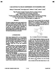
Fig. 1. Hash (left) and Saupe–MC (right) compressed Lenna images obtained with 1 and 2 seconds execution time repectively. It is arguable that the hash algorithm is “visually” better than MC–Saupe.

Following the standard quadtree approach, we will then divide the range in 4 subranges and try to code the subblocks with new domains of suitable size. We shall use this approach in our examples, with 16, 8 and 4 quadtree levels. Notice that a further 2 × 2 subdivision does not make sense, as the compression code requires by itself about 4 bytes. If a given 4 × 4 block cannot be compressed, we shall use JPEG DCT on its parent 8 × 8 block. In any case, these escapes are rare, less than 1 per thousand ranges. Notice that the preceding code uses two parameters, dM and dC , which clearly verify dM < dC . Ranges are compressed only if the minimal distance d verifies d < dC ; a good choice of dC is about 70% of the full image standard deviation, with 40 being an adequate value. The parameter dM is critical for the time perfomance of the algorithm, as it stops the time consuming block comparisons as soon as a good enough domain has been found (although, as mentioned before, may be not optimal). Of course, if dM is too large, it is likely that block comparisons will stop when a not too good domain has been examined. The result will be a fast algorithm but with low quality in the compressed image. On the other hand, a too small dM will give a good quality for the compressed image (or too many escape calls!) but it will also force possibly too many domains to be examined. A practical estimate is to set dM to about 70% of the average standard block deviation, with 8 being now an adequate value. We turn next to illustrate the application of hash FIC, comparing its performance with that of the Saupe–MC FIC.

38

36

PSNR

34

32

Saupe−MC Hash−like

30

28

0

0.5

1 bpp

1.5

2

Fig. 2. Rate–distortion curves for the hash (black points) and Saupe–MC algorithms. Both are similar up to 1 bpp, Saupe–MC being better afterwards, because of the earlier saturation of hash FIC (for better comparison, no escape calls have been used).

3

Experimental results

We will use for our comparisons the well known 512 × 512 Lenna image whose pixels have a 8 bit gray level. We shall work with a three–level quadtree with range sizes being 16 × 16, 8 × 8 and 4 × 4. When working with, say, 4 × 4 ranges, we shall use as domains all the 4 × 4 blocks in the decimated image with even coordinates of their upper left corner. This gives (128−4+1)2 '= 15.625 domains that become 125.000 after isometries are taken into account and 250.000 after adding the negative blocks. The number of hash points H is 5 and the maximum hash key value is thus 165 = 220 , resulting in a hash load factor of about 0.25. As mentioned before, the λ values used are 1.5 for 16 × 16 and 8 × 8 blocks, and 0.4 for 4 × 4 blocks. Other parameters of our hash FIC algorithm are dC = 40, dM = 8, C = 16, B = 8 and ∆ = 1. There has been much work done to define the “visual quality” of an image in terms of mathematical expressions [3]. We shall not use these measures here, but figure (1), corresponding to 1 second hash and 2 second Saupe–MC execution times, shows that the hash algorithm gives a rather good image quality, arguably better in this case than that of the Saupe–MC algorithm. Anyway, a more quantitative approach to measure the quality of a compression algorithm is to give the evolution with respect to execution time of either the compression rate achieved or the quality of the compressed image. Compresion rate is simply measured by the number of bits per pixel (bpp) in the new image. Image quality is measured by the peak signal to noise ratio PSNR, defined as 2552 ms error and measured in decibels (dBs). Figure (2) compares the rate–distortion, that is, the PSNR–bpp curves of the hash and Saupe–MC FIC. Clearly the algorithm P SN R = 10 log10

36

2

34 1.5

bpp

PSNR

32 1

30 Saupe MC Hash−like

0.5

28

26

0 0

2

4

t[s]

6

0

2

4

6

t[s]

Fig. 3. PSNR and bpp evolutions against execution time for the hash (black points) and Saupe–MC algorithms. Compressions are similar up to 4 seconds with hash giving smaller files after that and Saupe–MC higher PSNR. However the hash algorithm gives better results for small computing times, much better in fact below 2 seconds.

with a higher curve gives better results. As seen in the figure, both curves are equivalent up to a PSNR of about 33.5. After this value, the Saupe–MC curve is better. In fact, for high image quality compression (and therefore, large computing times), the Saupe–MC algorithm is bound to give somewhat better results. This is due to the fact that Saupe–MC uses an optimal block, while the hash algorithm stops domain searching once a close enough domain has been found. In any case, the well known JPEG algorithm will require smaller compression times than a FIC algorithm for high image quality, so the earlier PSNR saturation of the hash algorithm does not have a great practical relevance. Figure (3) gives PSNR and bpp time evolutions of the hash and Saupe–MC algorithms. Execution times are measured in a 800MHz Pentium III machine with 256 MB RAM. A higher PSNR curve is better and it is seen that here again Saupe-MC FIC gives better results in a high quality PSNR range. Notice that, however, below 3 seconds (or below a PSNR of 33), the hash PSNR curve is better, keeping in fact the same 33 PSNR down to 1 second. Moreover, while hash PSNR stays above 31 down to 0.5 seconds, Saupe-MC’s PSNR drops below 27 even with a 1.5 second execution time. The same figure shows similar compression rates up to 4 seconds. Above 4 seconds hash files are smaller but, as just seen, hash PSNR is lower. It follows from these images that for practical execution times, that is, below 3 seconds, the hash algorithm gives better results than Saupe–MC. Hash results are in fact much better for small execution times and lower quality ranges (as mentioned in [1] low quality image compression may be the most promising image processing area for FIC methods).

4

Conclusions and further work

To achieve linear execution time with respect to image size a FIC algorithm should make an average of O(1) full domain comparisons per each range to be compressed. In ordinary key search, hash algorithms can attain this performance and, ideally, the hash FIC method presented here could do so. In our experiments, typical average values for this are 3.9 domain comparisons per range when P SN R ' 33 and 3.1 comparisons when P SN R ' 27. The results shown here do support a linear execution time claim, at least in the low PSNR range, where our algorithm can be about 5 times faster than other state of the art acceleration schemes (excluding preparation and I/O times, it could be up to 10 times faster). Recall that as the hash algorithm does not guarantee using optimal domains, it is bound to give lower image quality for longer execution times. It is thus more appropriate to use it in the lower-quality range. There, the time performance of hash FIC makes it feasible to use it in real time compression. Interesting application areas for this could be the compression of images transmitted over mobile phones and even moving image compression, where foreground images would be used for domain codebooks. Another topic being considered is to introduce different block comparisons to get better image quality. In fact, a common problem of FIC algorithms is the presence of visual artifacts in the reconstructed image because of gray level overflows due to the linear nature of their range–domain approximation. This could be improved using non linear, saturating block comparison methods, for which hash FIC is well suited. The price to pay is, of course, longer execution times. With hash FIC, however, a non linear approach could be pursued, given the efficiency of the hash domain search. These and other application areas are currently being researched.

References 1. Y. Fisher, Fractal Image Compression–Theory and Application. New York: Springer–Verlag 1994. 2. B. Hurtgen and C. Stiller, “Fast hierarchical codebook search for fractal coding of still images”, in Proc. EOS/SPIE Visual Communications PACS Medical Applications ’93, Berlin, Germany, 1993. 3. M. Miyahara, K. Kotani and V.R. Algazi, “Objective picture quality scale (PQS) for image coding”, IEEE Trans. in Communications, vol. 46, pp. 1215–1226, 1998. 4. M. Polvere and M. Nappi, “Speed up in fractal image coding: comparison of methods”, IEEE Trans. Image Processing, vol. 9, pp. 1002–1009, June 2000. 5. D. Saupe, “Fractal image compression by multidimensional nearest neighbor search”, in Proc. DCC’95 Data Compression Conf., Mar. 1995.