and a Lipschitz-continuous pooling operator Pd. Convolu- tions with wavelet filters, ..... tion and entropy-based approach for systolic heart murmurs identification.
Heart Sound Classification Using Deep Structured Features Michael Tschannen, Thomas Kramer, Gian Marti, Matthias Heinzmann, Thomas Wiatowski Dept. IT & EE, ETH Zurich, Switzerland Abstract We present a novel machine learning-based method for heart sound classification which we submitted to the PhysioNet/CinC Challenge 2016. Our method relies on a robust feature representation—generated by a wavelet-based deep convolutional neural network (CNN)—of each cardiac cycle in the test recording, and support vector machine classification. In addition to the CNN-based features, our method incorporates physiological and spectral features to summarize the characteristics of the entire test recording. The proposed method obtained a score, sensitivity, and specificity of 0.812, 0.848, and 0.776, respectively, on the hidden challenge testing set.
1.
Introduction
Current state-of-the-art methods for automated classification of pathology in heart sound recordings often suffer from poor generalization capabilities because they were trained and/or evaluated on small and/or carefully selected data sets. The aim of the PhysioNet/CinC Challenge 2016 is to encourage the development of robust heart sound classification algorithms delivering accurate predictions in both real-world clinical and non-clinical environments [1]. In recent years, deep convolutional neural networks (CNNs) [2, 3] have proven to be tremendously successful in many practical classification tasks. By feeding the input signal through a sequence of modules—each of which computes a convolutional transform, a non-linearity, and a pooling operation—these networks extract features that incorporate signal characteristics important for discrimination (e.g., higher order moments [4]) while suppressing irrelevant variations (such as the temporal locations of signal characteristics [5, 6]). Although deep CNNs are often used to perform classification directly [2, 3], usually based on the output of the last network layer, they can also act as stand-alone feature extractors [7] with the extracted features fed into a classifier such as, e.g., a support vector machine (SVM). In this paper, we present a novel machine learning-based method for heart sound classification which we submitted to the PhysioNet/CinC Challenge 2016. The key ingredi-
ents of our method are a deep CNN-based feature extractor employing wavelet filters [8] and a SVM. By relying on pre-specified wavelet filters, instead of learning the filters from the data as in most standard deep CNN architectures, not only we decrease the training time drastically, but also we reduce the risk of overfitting due to the small training set at hand. We note that wavelet-based features in combination with a SVM have been considered previously for heart sound classification, e.g., in [9–11]. However, these methods employ the wavelet transform only, i.e., they can be considered as single layer CNNs without non-linearity and are hence “shallow”, whereas our “deep” approach employs wavelets as filters in a CNN (i.e., we employ wavelets and, additionally, non-linearities and pooling operations at multiple layers) to compute a rich and robust feature representation. For a more comprehensive review of prior work on heart sound classification we refer to [1, Sec. 3].
2.
Methods
Our method (see the illustration in Figure 1) consists of a feature extraction stage and a classification stage. In the former stage, two types of features are extracted from the test heart sound recording, namely “deep features” that provide a robust characterization of the shape and morphology of each cardiac cycle1 in the recording, and “summary features” that describe the entire recording. The extraction of deep features hence requires segmentation of the test recording into cardiac cycles. Each cardiac cycle is associated with the feature vector obtained by concatenating the corresponding deep features and the summary features (i.e., the summary features are shared across all feature vectors extracted from the test recording). In the classification stage, each feature vector is classified into {“normal”, “abnormal”} (and possibly “unsure”, due to poor signal quality) using a L2 -SVM with radial basis function (RBF) kernel, noting that the prediction for the entire recording is obtained as the majority vote over all cardiac cycles. The motivation for including summary features in ad1 The term “cardiac cycle” henceforth refers to the cardiac cycle itself or to the corresponding segment of the heart sound recording.
Figure 1. Illustration of the proposed method. dition to deep features is that classification based on deep features and majority voting alone may not sufficiently account for information that is spread over the entire recording such as, e.g., heart rate variability. The effect of summary features on the classification performance is numerically studied in Section 3. In the following, we describe all parts of our method in detail and discuss its evaluation and parameter selection. Segmentation: We use the heart sound segmentation algorithm from [12], which leverages a hidden semi-Markov model and Viterbi decoding to segment the test heart sound recording into the four heart sound states S1 (first heart sound), systole, S2 (second heart sound), and diastole. Deep features: We employ the tree-like CNN-based feature extractor proposed in [8], which we briefly review in the following. Every layer of the network—specified by the layer index 1 ≤ d ≤ D—is associated with a collection of pre-specified Haar wavelet filters2 {ψj }Jj=1 [13], a pointwise Lipschitz-continuous non-linearity ρd , and a Lipschitz-continuous pooling operator Pd . Convolutions with wavelet filters, besides allowing for an efficient implementation using the algorithme a` trous [13, Sec. 5.2.2], resolve characteristics of a signal at multiple scales 1 ≤ j ≤ J (respectively, signal characteristics that correspond to dyadic frequency bands [−2−(j−1) , −2−(j+1) ] ∪ [2−(j+1) , 2−(j−1) ]), the application of a pointwise nonlinearity ρd activates or de-activates features, and the application of a pooling operator Pd reduces the signal dimension and renders the features robust w.r.t. non-linear deformations and translations. Here, for all layers 1 ≤ d ≤ D, we use the rectified linear unit (ReLU) non-linearity and the max-pooling operator (see, e.g., [8, Sec. 2.2, 2.3] for definitions). Every layer of the network computes a set of d so-called feature maps {fnd }Jn=1 according to � �� d fnd := f(k,j) := Pd ρd fkd−1 ∗ ψj , (1) where 1 ≤ k ≤ J d−1 , 1 ≤ j ≤ J, f10 := f is the input signal (here, a cardiac cycle) fed into the network, and ∗ denotes the circular convolution operator. The underlying tree-like network architecture is illustrated in Figure 2. 2 The
networks considered in [8] allow for general frame filters.
The final feature vector describing f is obtained by collecting (in a single feature vector) (i) every feature map fnd , 1 ≤ d ≤ D, 1 ≤ n ≤ J d , generated in the network, (ii) low-pass filtered versions of the feature maps fnd , and (iii) a low-pass filtered version of the signal f itself. Figure 3 shows an example feature vector of a cardiac cycle for a network of depth D = 3 employing J = 3 wavelet scales, the network parameters used for the experiments in Section 3. P3 ρ3 f22 ∗ ψj2
��
2 P3 ρ3 f28 ∗ ψj2
P2 ρ2 f11 ∗ ψj1
��
P2 ρ2 f91 ∗ ψj3
P1 ρ1 f10 ∗ ψj1
��
P1 ρ1 f10 ∗ ψj3
��
��
��
f = f10
Figure 2. Tree-like deep CNN (of depth D = 3 employing J = 3 wavelet scales) underlying the feature extractor described in Section 2. The root of the network corresponds to d = 0. The signal fnd , defined in (1), corresponds to the n-th feature map in the d-th network layer. Before the cardiac cycles are fed into the feature extraction network, they are re-sampled to a length of 1024 to ensure that they are all mapped to feature vectors of equal dimension. Furthermore, each cardiac cycle is normalized by mean subtraction and division by its standard deviation. For the described network parameters the dimension of the feature vectors is 12,160. To reduce computational complexity (in particular during training) the dimension of the feature vectors is reduced to 400 by principal component analysis. Furthermore, the durations of the four heart sound states are appended to the (dimensionality-reduced) feature vectors as additional features. Preliminary experiments showed that the modulus nonlinearity and pooling by sub-sampling leads to marginally worse classification performance than the ReLU nonlinearity combined with max-pooling. These experiments also revealed that increasing the number of principal com-
2 1 0 −1 0
1
2
3
layer index Figure 3. Example feature vector generated by the deep CNN defined in Section 2. The 0-th layer corresponds to the low-pass filtered input cardiac cycle. ponents or the depth D of the feature extraction network does not significantly improve classification performance. Finally, an alternative to extract deep features from the 1-D cardiac cycles is to compute a 2-D time-frequency representation (e.g., a spectrogram) of the cardiac cycles and feeding them into our feature extraction network equipped with 2-D Haar wavelet filters (and, of course, 2-D pooling operators). Intuitively, such an approach might lead to a richer feature representation allowing for better discrimination between normal and abnormal heart sounds. However, preliminary experiments showed that this approach does not improve classification performance. Summary features (state statistics and PSD): We rely on the 20 features described in [1, Sec. 6.2] consisting of first and second order statistics of amplitudes and durations associated with the four heart sound states obtained through segmentation. We refer to this set of features as state statistics, see also Figure 1. In addition, we use a power spectral density (PSD) estimate of length 128 (covering the spectral band 0-500Hz) computed from the raw (unsegmented) heart sound recording using the Welch method [14, Sec. 2.7.2] with half-overlapping Hamming windows. The PSD estimate provides a compact description of the second order statistics of the heart sound recording and may improve the robustness of the classification when the segmentation is inaccurate. Evaluation and parameter selection: We evaluated the proposed method on the publicly available PhysioNet/CinC Challenge 2016 data set containing 3,153 heart sound recordings of 764 subjects, including both healthy individuals and patients with different heart diseases. Each recording has two labels, the first of which indicates whether the subject is healthy (“normal”) or was diagnosed with a cardiac disease (“abnormal”), and the second indicating the signal quality (“good”/“poor”). We refer the reader to [1] for a detailed description of the data set. The classification performance was assessed using the challenge score (MAcc) defined as the arithmetic mean of sensitivity and specificity, both modified to account for predictions of the label “unsure”, see [1, Eq. (1) and (2)] for details. We consider both binary classification into {“normal”, “abnormal”}, ignoring the quality
labels, and ternary classification into {“normal”, “abnormal”, “unsure”}, for which all the recordings with “poor” signal quality were labeled “unsure”. The parameter of the RBF kernel and the regularization parameter of the L2 -SVM were selected using 5-fold stratified (by patient) cross-validation. Class-adaptive sample weights were used to compensate for the class imbalance in the data set. Note that for ternary classification the sample weights were computed based on the labels “normal”/“abnormal” only as inclusion of the label “unsure” in the weight computation reduced the MAcc. Modification for unsupervised ternary classification: We briefly outline a simple modification (not used to obtain the results in Section 3) of our method to learn a ternary classifier based on the labels {“normal”, “abnormal”} only. Specifically, this extension implements a socalled reject option [15]. Assuming an estimate Pˆ (Y |r) of the posterior probability P (Y |r) of the label Y ∈ {“normal”, “abnormal”} given the test recording r to be available, a ternary prediction Yˆter is obtained as if Pˆ (Y = “abnormal”|r) < τ “normal”, ˆ Yter = “abnormal”, if Pˆ (Y = “abnormal”|r) > 1 − τ “unsure”, otherwise , where τ ∈ (0, 1/2] is a threshold parameter. Under certain (not necessarily realistic) model assumptions one can motivate the estimation of Pˆ (Y |r) according to Pˆ (Y |r) := PL (1/L) `=1 Pˆ (Y |b` ), where {b` }L `=1 are the cardiac cycles in the test recording r. With the heart sound classification method described above, the posterior probability estimates Pˆ (Y |b` ) can be obtained either from the SVM model using Platt scaling [16], or by replacing the SVM model with a logistic regression model. The threshold parameter τ can be optimized using cross-validation. If the score used to assess the performance of the classifier does not sufficiently reward the label “unsure”, τ = 0.5 will be selected, which amounts to binary classification.
3.
Results
Table 1 shows the 5-fold cross validation MAcc for binary and ternary classification. To study the effect of different features we report the performance for classification based on deep features only (DF), deep features and state statistics (DF + SS), as well as deep features and all summary features (DF + SS + PSD). The highest MAcc we obtained during the official phase of the PhysioNet/CinC Challenge 2016 on the hidden challenge testing set containing 1,277 recordings was 0.812 (sensitivity: 0.848, specificity: 0.776), for binary classification based on DF + SS + PSD. With this MAcc our algorithm is within 5.6% of the winning team’s MAcc, ranked 14th out of 48 competitors. In terms of running time, all
our entries to the challenge during the official phase used less than 21% of the computation quota available.
features DF DF + SS DF + SS + PSD DF DF + SS DF + SS + PSD
binary classification MAcc Se Sp 0.854 0.869 0.838 0.860 0.910 0.811 0.870 0.908 0.832 ternary classification 0.845 0.844 0.847 0.847 0.841 0.854 0.855 0.847 0.863
[2] [3]
[4]
[5] [6]
Table 1. Results (MAcc: challenge score, Se: sensitivity, Sp: specificity) for different configurations of our method (5-fold cross validation).
4.
[7]
Discussion
For binary classification, the results in Table 1 show that a combination of deep features and summary features leads to a higher MAcc than purely deep feature-based classification. In more detail, the configurations involving summary features have a slightly lower specificity and a significantly higher sensitivity than the configuration based on deep features only, hence leading to less balance between sensitivity and specificity. For ternary classification, the improvement through summary features is less pronounced than for binary classification. Perhaps surprisingly, ternary classification consistently leads to a lower MAcc than binary classification. Possible reasons for this phenomenon could be that the subset of recordings with “poor” signal quality is too heterogeneous to be reliably discriminated from “normal” and “abnormal” recordings using our method, or that reliable classification into {“normal”, “abnormal”} is sometimes possible even when a recording has “poor” signal quality.
[8]
[9]
[10]
[11]
[12]
[13]
5.
Conclusion
We presented and evaluated a robust method for heart sound classification that combines a deep CNN-based feature extractor and a SVM. Improving the identification of recordings with poor signal quality and a more elaborate way to incorporate summary features into the proposed method are interesting directions to be explored in the future.
References [1]
Liu C, Springer D, Li Q, Moody B, Juan RA, Chorro FJ, Castells F, Roig JM, Silva I, Johnson AE, Syed Z, Schmidt SE, Papadaniil CD, Hadjileontiadis L, Naseri H, Moukadem A, Dieterlen A, Brandt C, Tang H, Samieinasab M,
[14] [15] [16]
Samieinasab MR, Sameni R, Mark RG, Clifford GD. An open access database for the evaluation of heart sound algorithms. Physiological Measurement 2016;37(11). LeCun Y, Bengio Y, Hinton G. Deep learning. Nature 2015; 521(7553):436–444. Goodfellow I, Bengio Y, Courville A. Deep learning, 2016. URL http://www.deeplearningbook.org. Book in preparation for MIT Press. Bruna J, Mallat S. Invariant scattering convolution networks. IEEE Transactions on Pattern Analysis and Machine Intelligence 2013;35(8):1872–1886. Mallat S. Group invariant scattering. Communications on Pure and Applied Mathematics 2012;65(10):1331–1398. Wiatowski T, B¨olcskei H. A mathematical theory of deep convolutional neural networks for feature extraction. arXiv151206293 2015;. Huang FJ, LeCun Y. Large-scale learning with SVM and convolutional nets for generic object categorization. In Proc. of IEEE International Conference on Computer Vision and Pattern Recognition. 2006; 284–291. Wiatowski T, Tschannen M, Stani´c A, Grohs P, B¨olcskei H. Discrete deep feature extraction: A theory and new architectures. In Proc. of International Conference on Machine Learning. June 2016; 2149–2158. Ari S, Hembram K, Saha G. Detection of cardiac abnormality from PCG signal using LMS based least square svm classifier. Expert Systems with Applications 2010; 37(12):8019–8026. Patidar S, Pachori RB, Garg N. Automatic diagnosis of septal defects based on tunable-Q wavelet transform of cardiac sound signals. Expert Systems with Applications 2015; 42(7):3315–3326. Zheng Y, Guo X, Ding X. A novel hybrid energy fraction and entropy-based approach for systolic heart murmurs identification. Expert Systems with Applications 2015; 42(5):2710–2721. Springer DB, Tarassenko L, Clifford GD. Logistic regression-HSMM-based heart sound segmentation. IEEE Transactions on Biomedical Engineering 2016;63(4):822– 832. Mallat S. A wavelet tour of signal processing: The sparse way. 3rd edition. Academic Press, 2009. Stoica P, Moses RL. Spectral analysis of signals. Pearson/Prentice Hall Upper Saddle River, NJ, 2005. Herbei R, Wegkamp MH. Classification with reject option. Canadian Journal of Statistics 2006;34(4):709–721. Platt J. Probabilistic outputs for support vector machines and comparisons to regularized likelihood methods. Advances in Large Margin Classifiers 1999;10(3):61–74.
Address for correspondence: Michael Tschannen, Thomas Wiatowski ETH Z¨urich, Communication Technology Laboratory Sternwartstrasse 7 CH-8092 Z¨urich Switzerland {michaelt, withomas}@nari.ee.ethz.ch