in Harvard's Division of Applied Science and one ... computer company: software development, quality ..... degree in Com
Heuristic Cleaning Algorithms in Log-Structured File Systems Trevor Blackwell, Jeffrey Harris, Margo Seltzer Harvard University
Abstract Research results show that while LogStructured File Systems (LFS) offer the potential for dramatically improved file system performance, the cleaner can seriously degrade performance, by as much as 40% in transaction processing workloads [9]. Our goal is to examine trace data from live file systems and use those to derive simple heuristics that will permit the cleaner to run without interfering with normal file access. Our results show that trivial heuristics perform very well, allowing 97% of all cleaning on the most heavily loaded system we studied to be done in the background.
1.
Introduction
The Log-Structured File System is a novel disk storage system that performs all disk writes contiguously. Since this rids the system of seeks during writing, the potential performance of such a system is much greater than in the standard Fast File System [4], which must make writes to several different locations on the disk for common operations such as file creation. The mechanism used by LFS to provide sequential writing is to treat the disk as a log composed of a collection of large (one-half to one megabyte) segments, each of which is written sequentially. New and modified data are appended to the end of this log. Since this is an append-only system, all the segments in the file system eventually become full. However, as data are updated or deleted, blocks that reside in the log become replaced or removed and their space can be reclaimed. This reclamation of space, gathering the freed blocks into clean segments, is called cleaning and is a form of generational garbage collection [3]. The critical challenge for LFS in providing high performance is to keep cleaning overhead
low, and more importantly, to ensure that I/Os associated with cleaning do not interfere with normal file system activity. There are three terms that will be useful in discussing LFS cleaner performance write cost, ondemand cleaning, and background cleaning. Rosenblum defines write cost as the average amount of time that the disk is busy per byte of new data written, including all the cleaning overheads [8]. A write cost of 1.0 is perfect meaning that data can be written at the full disk bandwidth and never touched again. A write cost of 10.0 means that writes are ultimately performed at one-tenth the maximum bandwidth. A write cost above 1.0 indicates that data had to be cleaned, that is, rewritten to another segment in order to reclaim space. Cleaning is performed for one of two reasons: either the file system becomes full, in which case cleaning is required before more data can be written, or the file system becomes lightly utilized and can be cleaned without adversely affecting normal activity. We call the first case when the cleaner is required to run, ondemand cleaning and the latter, optionally running the cleaner, background cleaning. Using these three terms, we can restate the challenge of LFS as minimizing write cost and avoiding on-demand cleaning. The cleaning behavior of Sprite-LFS was monitored over a four-month period [8]. The measurements indicated that one-half of the segments cleaned during a four month period were empty and that the maximum write-cost observed in their environment was 1.6. While this write cost is acceptably low, the results do not give an indication of the impact on file system latency that resulted from cleaner I/Os interfering with user I/Os. Seltzer et al. report that cleaning overheads can be substantial, as
much as 41% in a transaction processing environment [9]. However, the cleaning cost in a benchmarking environment is an unrealistic indicator since the benchmark is constantly demanding use of the file system. Unlike benchmark environments, the realworld behavior of most workstation environments is observed to be bursty [1][5]. For example, consider an application that has two phases in which it executes. In phase 1, it creates and deletes many small files. In phase 2, it computes or uses the network, or terminates. Examples of such applications include Sendmail and NNTP servers. In FFS, the writes for the new data are all performed at the time the creates and deletes are issued. In LFS, all the small writes are bundled together into large, contiguous writes, so bandwidth utilization exceeds 50%, and approaches 100% as file size increases. The cleaner can run during the non-disk phase of the application when it does not interfere with application I/O. This workload is diagrammed in Figure 1. The goal of this work is to investigate the real cost of cleaning, in terms of user-perceived latency. Using trace data gathered from three file servers, we have found that simple heuristics enable us to remove nearly all on-demand cleaning (specifically, on the most heavily loaded system, only 3.3% of the cleaning had to be done on-demand). The target operating environment of this study is a conventional UNIX-based network of workstations where files are stored on one or more shared file servers. These results do not necessarily hold for all environments; Time
FFS
CPU Network Disk
Sync. Writes LFS
CPU Network Disk
Log Cleaning Writes
Cleaning
Figure 1. Overlapping cleaning with non-disk activity. The two traces depict FFS and LFS processing cycles. Both systems are writing the same amount of data, but FFS must issue its writes synchronously, resulting in a much longer total execution time. LFS issues its write asynchronously and cleans during processing periods, thus achieving much shorter total execution time.
they may not apply to online transaction processing environments where peak or near-peak transaction rates must be sustained at all times. Section 2 describes the environments in which we gathered our measurements, Section 3 describes the traces we gathered, and Section 4 describes the tools and simulation model we used. Section 5 presents the results of our simulations, and Section 6 discusses the conclusions and ramifications of this work.
2.
Benchmarking Methodology
All our trace data was collected by monitoring NFS packets to servers that provide only remote access. The NFSWatch utility [10], present on many UNIX systems, monitors all network traffic to an NFS file server and categorizes it, periodically displaying the number and percentage of packets received for each type of NFS operation. We modified the tool to output a log record for every NFS request. Since NFSWatch snoops on the ethernet, it does not capture local activity to a disk. To guarantee that we capture all activity to the file systems under study, we have limited our analysis to three Network Appliance FAServers [2], which are not general-purpose machines and provide no disk traffic other than serving NFS requests. An issue in using Ethernet snooping is the potential for packet loss at the snooping host, which could skew the results. To detect such occurrences, we ran a daemon on a client host which referenced an unusually named file every 6 minutes. We could then search the log to find missing records. Only two lost requests out of 2200 were detected, indicating that the traces are fairly accurate. The lost packets were both at times of heavy demand, so while this form of loss may cause a slight underestimate of total traffic, it does not affect our estimates of idle time. Two of the FAServers (Attic and Cellar) reside in Harvard’s Division of Applied Science and one (Maytag) resides at Network Appliance’s Corporate Headquarters. The Harvard environment consists of approximately 90 varied workstations (e.g. HP, DEC, SUN, X86) and X-terminals on two Ethernets. The DAS user community consists of approximately 100 users, most of whom use UNIX systems for text processing, email, news, software development, simulation, trace-gathering, and a variety of researchrelated activities. The Network Appliance environment consists of 90 workstations (mostly
Sparcstations,) X-terminals, PCs, and Macintoshes; the servers and some clients are on an FDDI ring. These machines service all business aspects of a small computer company: software development, quality assurance, manufacturing, MIS, marketing, and administration. The Network Appliance user community is approximately 60 users, of which 15-20 are heavy UNIX users, another 5-10 are casual users and the remaining use the PCs and Macintoshes nearly exclusively, placing little load on the NFS servers.
Machine Type
Harvard DAS (Attic and Cellar)
Network Appliance (Maytag)
Clients Servers Clients Servers HP700
9
1
0
0
Sun 3
0
2
0
0
SparcStations
38
2
15
2
DEC Alphas
5
1
0
0
DEC MIPS
4
0
0
0
FAServer
0
2
0
3
x86 (DOS and UNIX)
6
1
17
5
SGI
3
0
1
0
Macintosh
1
0
31
0
NeXT
5
0
0
0
Router terminal concentrators
5
0
2
0
X-Terminals
12
0
13
0
Total
88
9
79
10
Table 1. Measurement Environment. This table shows the per-machine-type breakdown of both the DAS and Network Appliance environments.
Table 1 summarizes our measurement environments. The client column indicates how many of the machines do not serve any files while the server column indicates how many of the machines act as NFS servers. The eight servers in the Harvard environment serve approximately 50 file systems. The nine servers in the Network Appliance environment serve approximately eleven file systems.
3.
The Traces
We modified NFSWatch to log each operation, recording a timestamp, the sender’s IP address, the server’s IP address, packet size, request type, and request specific information. The request-specific information identifies the file being accessed, the offset in the file, and the number of bytes. The traces were gathered for 24 hours per day for several days (9 for Attic, 12 for Cellar, and 2.5 for Maytag). The Maytag traces would have been longer, but crashes of the tracing machine at Network Appliance prevented us from gathering a single, longer trace. Table 2 summarizes the file system activity during the trace period. Characteristic
Attic
Cellar
Maytag
Total Requests
4.0 M
1.5 M
7.5 M
Data Read Requests
835 K
177 K
495 K
Reads from Cache
20.3 GB
8.9 GB
36.6 GB
Reads from Disk
7.1 GB
1.1 GB
3.4 GB
Data Write Requests
349 K
194 K
330 K
User Writes to Disk
3.4 GB
1.5 GB
5.5 GB
Directory Reads lookup, readdir
1.9 M
0.9 M
2.3 M
Directory Modifications create, mkdir, rm, rename, rmdir
43 K
13 K
410 K
Inode Updates
427 K
215 K
764 K
Trace Length
9 days
16 days
2.5 days
File System Size
4 GB
1 GB
8 GB
Disk Space Utilization
90%
90%
90%
Table 2. Summary of trace data collected on the three FAServers. All traces were gathered using the NFSWatch utility. We adjusted the disk sizes to achieve 90% utilization through most of the traces.
Because we gathered the trace data by capturing NFS requests, there are a few limitations in our data. The NFS_CREAT call returns an inode number (as part of the file handle) which is not captured by our trace gathering tools. In order to determine which inode was created in response to the NFS_CREAT call, we perform a look-ahead to the next NFS_WRITE or NFS_SETATTR call from the same client for the same file system and assume it belongs to the newly created inode. There are only two cases that are problematic: the creation of two or
more files in rapid succession by the same client and the creation of a file which is not immediately written, and whose attributes are not set. Both of these cases are detectable and a pass over our traces reveals that we correctly matched the NFS_CREAT with the inode number 99% of the time NFS caching differs from local file system caching. Since NFS client caches timeout, we record requests at the server that would normally be satisfied by the local filesystem buffer cache. However, since we model a large (10 MB) cache on the server, this phenomenon does not affect results of disk behavior. Another artifact of NFS is that writes can arrive at the server in bursts corresponding to the number of biods running on the client. As will be discussed in Section 4, we model two different protocols for writing the NFS requests. These different models allow us to emulate both NFS and local file system behavior. The shortcomings of using NFS as our tracegathering method are outweighed by its advantages. By examining traffic on the local Ethernets, our tracing has no effect on the data gathered (our trace files are not written to the servers under examination). Other tracing methods that run on the server itself would not provide this unobtrusiveness.
4.
The Simulator
We analyzed LFS behavior by simulating an LFS file system for each server. The simulator consists of approximately 4000 lines of ParcPlace Smalltalk in 55 classes. The simulator maintains a ten megabyte cache of in-memory blocks and maintains counts of the number of operations requested, the cache hit rate, the number and placement of I/Os in response to NFS requests, and the number of sectors read and written for on-demand and background cleaning. In addition, a graphical display depicts the file system during simulation, enabling the user to visualize file layout, data expiration, and cleaning. The simulator processes trace records at a rate of approximately 1000 records per second (half that if the graphical display is updated frequently). If desired, the simulation can be slowed sufficiently that every disk access can be observed graphically. Since we are analyzing a live file system, we must create an equivalent LFS version of the file system as it exists before our tracing begins. We can then apply our trace data to this initial state. Since the file system under study is not an actual LFS, we must process the existing initial configuration and create an
LFS that realistically depicts the file layout one would expect on a LFS. The main point of interest in the initial state is how files are distributed across segments. In an ideal configuration, each file would be allocated contiguously on disk and all files smaller than a segment would reside within the same segment. In reality, files may be distributed across multiple segments because of the order in which writes occur. If writes to many different files are intermixed, then segments may contain parts of several files. In order to create a realistic initial state, we use the timing of NFS operations in the actual traces to provide an indicator of how much files should be interleaved in the initial state. Before tracing, we snapshot the file system to record the size of every file. We group the files into bins based on the log2 of the number of blocks in the file. We then process the traces to compute the average number of segments spanned by files of each bin size. Finally, we take each file in the initial configuration and distribute it evenly to the average number of segments spanned by files of its size. Within a segment, we allocate files sequentially. In this manner, we create an initial configuration consistent with the data gathered in our traces. To reduce the memory requirements of the simulation, files that are never referenced during the trace do not have space allocated for them on the disk. The simulator provides a high-level model of LFS. It maintains file objects that record the location of their blocks, and directory objects that contain lists of the files they contain. The inode map, which maps inode numbers to the disk blocks in which they reside [7], is not directly simulated. Instead, each file is assessed 16 bytes of overhead in addition to the blocks that comprise it; this overhead is written as part of the segment summary. The servers simulate a ten megabyte leastrecently-used cache of data blocks, directory data, and inodes. If requested data are present in the cache, the request is serviced immediately and no disk operation is invoked. If the data are not present, then a disk request is scheduled. The simulator reads each trace record and examines the operation type. If the record is a read operation (either data or meta-data), the simulator consults the appropriate object and determines if the required data are in the cache. If they are, the referenced data are made most-recently-used (MRU). If they are not, a disk request is recorded and the new
blocks are added to the cache. If the request is a write, then the data are added to the current segment, the old copy of the data (if it exists) is marked invalid in the in-memory representation of the disk map, and the simulator counters are updated. In a real LFS data are not explicitly marked invalid; instead the number of live bytes are maintained per segment and the cleaner detects invalid blocks by consulting the file meta-data (i.e. inode). Our explicit marking of data does not change the behavior of cleaning, it merely simplifies our implementation. We simulate two write algorithms The first, called NFS-async, does not provide synchronous NFS semantics. It assumes that either the file systems are mounted with the unsafe NFS option [6] or that the system is equipped with at least two segments worth of non-volatile RAM into which segments are written before they are transferred to disk. In either case, the system caches data until a full segment accumulates before writing it to disk. The second model, NFSsynch, supports the synchronous behavior of NFS by writing a partial segment for each operation.
5.
Results
Our results fall into three categories. First, we examine the behavior of the disk system, analyzing the frequency and length of idle intervals. The distribution of idle intervals indicates what heuristics will be effective for initiating the cleaner. Using these heuristics, we then examine how much data accumulates between cleaner invocations. This determines the maximum disk utilization that should be employed to avoid cleaner interference with normal disk activity. Finally, we examine the disk queue lengths that arise, giving an indication of the latency observed by the clients.
5.1. Idle Time Distribution During the simulation, we recorded statistics on the length of idle intervals at the disk. For each of the servers under study, Figure 2 shows the distribution of intervals during which the disk was idle under the NFS-async model. We have removed all idle gaps of less than one second since these intervals predominate, but are sufficiently short that the cleaner will never run in them. The important feature of these distributions is that while most gaps were small (less than 1 second and not depicted in Figure 2) the absolute number of large intervals is sufficient to perform cleaning. More importantly, a long interval (greater than 2 seconds) is a good predictor of an even longer interval (greater than 4 seconds). For our file systems
using the asynchronous NFS algorithm, the probability that an idle period is at least four seconds long, once it is already two seconds long is more than 95% (96% on Attic, 97% on Cellar, and 98% on Maytag). Because cleaner and user disk accesses are identified as such in our simulated disk queue, we were able to compute another measure of cleaning impact: the average number of cleaner writes in the queue when a user write was added to the queue. Table 3 shows the results, which indicate that interference is minimal - at most 0.07 requests. System
Model
Interference
NFS-sync
0.069
NFS-async
0.067
NFS-sync
0.057
NFS-async
0.072
NFS-sync
0.039
NFS-async
0.022
Attic
Cellar
Maytag
Table 3. Cleaner Interference. Interference numbers are the average number of cleaner requests in the disk queue when a user request is added. These numbers place an upper bound on the amount of cleaner interference with user activity. Cleaner activity writes to the same part of the disk as user activity, so often cleaner writes can be scheduled along with user writes without a major performance impact.
Figure 3 shows the same distributions as Figure 2, but for the NFS-sync model. In this case, each NFS request that changes the file system (create, write, mkdir, rm, rmdir, rename, setattr) is written to disk as a partial segment. This reduces the number of long idle gaps and also increases the need for cleaning since each partial segment introduces 512 bytes of overhead for at most eight kilobytes of data. Still, the probability that a two second interval is a good predictor for an interval greater than four seconds is still high (96% on Attic, 98% on Cellar, and 86% on Maytag). The gradual slopes in the cumulative distributions shown in Figure 2 emphasize this phenomena. Despite the fact that Maytag seems to have the highest chance of cleaner activity being interrupted, the data in Table 3 shows that the interference is the least of the file systems. The cleaner on Maytag was generally able to clean less-utilized segments than on
Attic (NFS-async)
Attic (NFS-sync) 100000 Number of Gaps (log scale)
Number of Gaps (log scale)
100000 10000 1000 100 10 1
10000 1000 100 10 1
0
50
100 150 200 Gap Length (seconds)
250
300
0
50
Cellar (NFS-async)
300
250
300
250
300
100000 Number of Gaps (log scale)
Number of Gaps (log scale)
250
Cellar (NFS-sync)
100000 10000 1000 100 10 1
10000 1000 100 10 1
0
50
100 150 200 Gap Length (seconds)
250
300
0
50
100 150 200 Gap Length (seconds)
Maytag (NFS-sync)
Maytag (NFS-async)
100000 Number of Gaps (log scale)
100000 Number of Gaps (log scale)
100 150 200 Gap Length (seconds)
10000 1000 100 10
10000 1000 100 10 1
1 0
50
100 150 200 Gap Length (seconds)
250
300
Figure 2. Idle Time Distributions for NFS-async. The three graphs show the distribution of idle disk intervals for each server. While most gaps are very short (the number of gaps less than 1 second completely dominates the distribution and has been omitted from these graphs), there are a sufficient number of large idle intervals that background cleaning can be performed frequently. The bump in Attic’s trace at 120 seconds probably indicates a periodic process which often terminated an idle interval by performing some activity every 2 minutes.
0
50
100 150 200 Gap Length (seconds)
Figure 3. Idle Time Distributions for NFS-sync. These distributions show similar behavior to those in Figure 2 but with a steeper curve. Since writes are sent to the disk immediately upon their arrival, there are more individual requests to the disk, the disk is used less efficiently and there are more shorter idle intervals. Even so, using a two second gap as a predictor is an effective heuristic for finding gaps that are large enough to permit cleaning of at least one segment.
• Mark the segment clean.
All Servers (NFS-async) Cumulative Percentage of Gaps
100% Attic Cellar Maytag
80% 60% 40% 20% 0% 1
2
4
8 16 32 64 Gap Length (seconds)
128
256
All Servers (NFS-sync) Cumulative Percentage of Gaps
100% Attic Cellar Maytag
80% 60% 40%
The two long-running steps in this algorithm are the first, reading one megabyte from disk, and third, rewriting data into the log. In the pessimistic case, the read of the old segment will be a one megabyte sequential read, which takes well under a second on most of today’s disks (e.g. a DSP 3501 SCSI disk can read 1 MB in approximately one-half second). Frequently, there will be few enough live bytes in the segment that we can avoid reading the entire segment and only read the blocks that need to be cleaned. The write time depends on the utilization of the segment being cleaned. If the segment utilization is very high, then we may need to write most of a megabyte; if the segment is lightly utilized, we can write only a few blocks. Even in the worst case, a one megabyte write takes only 0.75 seconds on the DSP 3501. In this worst case, we can clean at a rate of one segment per 1.25 seconds and in most cases, we can clean at a substantially higher rate. Therefore, if we use the two second idle time predictor, more than 90% of the time the cleaner will complete at least one segment’s worth of cleaning before any user requests arrive.
20% 0% 1
2
4
8 16 32 64 Gap Length (seconds)
128
256
Figure 4. Cumulative Idle Time distributions. The gentle slope of the cumulative distributions between two and four second gaps emphasizes the predictive nature of two second gaps. Although most gaps are quite small (all gaps less than one second have been omitted from these distributions as is the case in the previous figures), there are still a sufficient number of large intervals in which to clean. Attic or Cellar; the smaller average size of cleaner writes is responsible for the lower cleaner interference. To understand how we can fit cleaning into these gaps, we need to quantify the time required to clean. In the best case, cleaning is free because there are segments that have no live data remaining in them (they are easily identified because we keep a count of the number of live bytes in each segment). In the general case, cleaning is summarized by the following algorithm. • Read a segment from disk.
Using this algorithm on our trace data, we found that we were able to use only background cleaning on Attic and Cellar (although disk utilization was 90% on all three servers, Attic and Cellar never ran sufficiently close to the file system capacity that on-demand cleaning was triggered). Maytag required occasional on-demand cleaning — 3.3% of the total number of segments cleaned were on-demand.
5.2. Dirty Data Accumulation Figure 5 shows the distribution of dirty data accumulation between cleaning intervals in the NFSasync model and Figure 6 shows the distributions in the NFS-sync model. The cumulative distributions are shown in Figure 7. On Maytag, the most heavily utilized system, the write volume due to user requests was about 2.2 GB per day. Running the cleaner to generate 2.2 GB of clean segments takes no more than 2750 seconds on the DSP 3501 disk - in practice, we estimate it to take about one third of this time on average. The large number of significant idle gaps during the day allowed cleaning to occur many times during the day, so that large quantities of unclean segments did not accumulate.
• Determine which blocks are live. • Append the live blocks to the end of the log.
The cumulative distributions shown Figure 7 illustrate how rarely large amounts of data are written
Attic (NFS-async)
Attic (NFS-async) 10000
Occurrences (log scale)
Occurrences (log scale)
10000
1000
100
10
1
1000
100
10
1 1
2
4
8 16 32 64 Data Written (MB)
128 256 512
1
2
4
Cellar (NFS-async) 10000
1000
Occurrences (log scale)
Occurrences (log scale)
128 256 512
Cellar (NFS-sync)
10000
100
10
1
1000
100
10
1 1
2
4
8 16 32 64 Data Written (MB)
128 256 512
1
2
4
Maytag (NFS-async)
8 16 32 64 Data Written (MB)
128 256 512
Maytag (NFS-sync) 10000
Occurrences (log scale)
10000
Occurrences (log scale)
8 16 32 64 Data Written (MB)
1000
100
10
1
1000
100
10
1 1
2
4
8 16 32 64 Data Written (MB)
128 256 512
Figure 5. Distributions of Accumulated Dirty Data in the NFS-async model. Except for a few occurrences, the the amount of data written before cleaning was possible was small - less than 100 MB. On a multi-gigabyte file system that is limited to 90% fullness, there is plenty of space for accomodating this amount of data without requiring on-demand cleaning. We never observed more than 350 MB (4.5% of Maytag’s disk space) written before cleaning occurred.
1
2
4
8 16 32 64 Data Written (MB)
128 256 512
Figure 6. Distributions of Accumulated Dirty Data in the NFS-sync model. In the NFS-sync model, we never observed more than 420 MB (5.2% of Maytag’s disk space) written before cleaning occurred.
Attic (NFS-sync) 10000
99%
Attic Cellar Maytag
98% 97% 96%
Number of Requests (log scale)
Cumulative Percentage of Occurrences
All Servers (NFS-async) 100%
1000
100
10
1 95% 1
2
4 8 16 32 64 128 256 512 Data Written Before Clean (MB)
0
1000
Cellar (NFS-sync) 10000
Attic Cellar Maytag
99% 98% 97% 96%
Number of Requests (log scale)
100%
1000
100
10
1 95% 1
2
4 8 16 32 64 128 256 512 Data Written Before Clean (MB)
Figure 7. Cumulative Distributions of Dirty Data Accumulation. Note that the range of the graph starts at 95%. The vast majority (96%) of all write bursts are small (less than 1 MB). Despite the substantial difference in the average traffic levels to these machines, the distribution of many-megabyte bursts of write activity is similar. before cleaning can be done. More than 96% of writes are less than one megabyte; 99% are less than four megabytes. This is true across all file systems studied.
5.3. Queueing Delays The last area of investigation is the queuing delays observed at the disk. Log-structured file systems use the disk system efficiently by issuing large, sequential transfers. If the disk is being used efficiently, queueing delays should be kept to a minimum. However, large transfers also keep the disk busy for long bursts of time. Incoming requests that get queued after one of these long writes can wait for a long time. Figure 8 shows the queuing delays observed for the NFS-async model and Figure 9 shows the queueing delays for the NFS-sync model. The cumulative distributions are shown in Figure 10.
0
200 400 600 800 Queuing Delay (milliseconds)
1000
Maytag (NFS-sync) 10000 Number of Requests (log scale)
Cumulative Percentage of Occurrences
All Servers (NFS-sync)
200 400 600 800 Queuing Delay (milliseconds)
1000
100
10
1 0
200 400 600 800 Queuing Delay (milliseconds)
1000
Figure 8. Distribution of Queueing Delays in the NFS-sync model. Comparing the two models, it is evident that delays are frequently longer in the NFSsync case.
Attic (NFS-async)
All Servers (NFS-async) 100% Cumulative Percentage of Delays
Number of Requests (log scale)
10000
1000
100
10
1
80% 60% 40% 20%
Attic Cellar Maytag
0% 0
200 400 600 800 Queuing Delay (milliseconds)
1000
1
Cellar (NFS-async) 100% Cumulative Percentage of Delays
Number of Requests (log scale)
1000
All Servers (NFS-sync)
10000
1000
100
10
1
80% 60% 40% 20%
Attic Cellar Maytag
0% 0
200 400 600 800 Queuing Delay (milliseconds)
1000
1
10 100 Queuing Delay (milliseconds)
1000
Figure 10. Cumulative Distributions for Queueing Delays. For all systems, more than 70% of the delays were zero, i.e. the request was put on an otherwise empty disk queue. Delays in the NFS-sync model were generally longer, probably due to both the increased write volume, and the fact that all writes for one request must complete before writes for another begin, which increases the number of rotational latencies incurred between writes.
Maytag (NFS-async) 10000 Number of Requests (log scale)
10 100 Queuing Delay (milliseconds)
1000
100
10
1 0
200 400 600 800 Queuing Delay (milliseconds)
1000
Figure 9. Distribution of Queueing Delays in the NFS-async model. Although there were occasional occurrences of large delays, most of the delays were small.
All three file systems under both models could service the majority of requests with no queuing delay at all. Delays in the NFS-sync model were generally longer, due to both the increased write volume, and the fact that all writes for one request must complete before writes for another begin, which increases the number of rotational latencies incurred between writes. Because our traces capture the time at which interactions happened between real clients and servers, the interval between closely spaced operations depends strongly on the speed of the real servers, as clients generally limit their maximum number of outstanding requests. To the extent that our
simulated file systems were faster or slower for various operations, the queuing delay may not be representative of a real system. However, the differences between NFS-sync and NFS-async reflect a real performance difference.
6.
Lieberman, H., Hewitt, C., “A real-time garbage collector based on the lifetimes of objects,” Communications of the ACM, 26, 6, 1983, 419-429.
[4]
McKusick, M.Joy, W., Leffler, S., Fabry, R. “A Fast File System for UNIX, “Transactions on Computer Systems 2, 3 (August 1984), pp 181197.
[5]
Ousterhout, J., Costa, H., Harrison, D., Kunze, J., Kupfer, M., Thompson, J., “A Trace-Driven Analysis of the UNIX 4.2BSD File System,’” Proceedings of the Tenth Symposium on Operating System Principles, December 1985, 1524.
[6]
Pawlowski, B., Juszczak, C., Staubach, P., Smith, C., Lebel, D., Hitz., D., “NFS Version 3: Design and Implementation,” Proceedings of the 1994 Summer Usenix Conference, Boston, MA, June 1994, 137-152.
[7]
Rosenblum, M., Ousterhout, J., “The LFS Storage Manager,” Proceedings of the 1990 Summer Usenix, Anaheim, CA, June 1990.
[8]
Rosenblum, M. and Ousterhout, J. ``The Design and Implementation of a Log-Structured File System.” ACM Transactions on Computer Systems, 10, 1 (February 1992), pp. 26-52.
[9]
Seltzer, M., Bostic, K., McKusick, M.K., and Staelin, C. ``An Implementation of a LogStructured File System for UNIX.” Proceedings of the 1993 Winter USENIX Conference, January 1993, pp. 307-326.
[10]
SunOS System Administrator’s Reference Manual, Section 8L.
Conclusions
The simulation results are very encouraging for LFS. With a simple heuristic of cleaning whenever the disk has been idle for two seconds, we can virtually eliminate any user-perceived cleaning latency. Only a very small portion of disk queue latency is due to cleaner activity. Our results hold across two different environments: a university research environment and a commercial product development environment. However, some workloads (e.g. online transaction processing) may not demonstrate the idle-gap distribution on which this heuristic depends. In these cases, log-structured file systems must rely on other cleaning solutions [9].
7.
[3]
Availability
The final trace set and the simulator software will be made available via Mosaic, at the URL: http://das-www.harvard.edu/users/students/ Trevor_Blackwell/Usenix95.html
8.
Acknowledgments
We gratefully thank Network Appliance for providing us our first FAServer and for graciously running our tracing tools to enable us to provide trace data from very different environments. We also thank Hewlett Packard for the equipment grant that provided disk space on which to store our trace data and many, many CPU cycles for simulation. This work was funded in part by NSF grant CDA-94-01024.
9.
References
[1]
Baker, M., Hartman., J., Kupfer., M., Shirriff, L., Ousterhout, J., “Measurements of a Distributed File System,’’ Proceedings of the 13th Symposium on Operating System Principles, Monterey, CA, October 1991, 198-212.
[2]
Hitz, D., Lau, J., Malcolm, M., “File System Design for an NFS File Server Appliance,” Proceedings of the 1994 Winter Usenix, San Francisco, CA, January 1994, pp. 235-246.
Trevor L. Blackwell is a graduate student of Computer Science in the Division of Applied Sciences at Harvard University. His research interests include gigabit network design, efficient signalling protocol implementation, and wireless networking. He has worked at Bell-Northern Research since 1988, is currently supported at Harvard by BNR’s External Research program. He was the recipient of a Canada Scholarship and IEEE McNaughton Scholarship. Blackwell received a B.Eng from Carleton University, Ottawa, in 1992. He can be reached at
[email protected]. Jeffrey J. Harris is an undergraduate student of Computer Science in the Division of Applied Sciences at Harvard University. His research interests
include memory management systems, and the application of non-volatile memory to file systems. He has worked previously with Dr. Seltzer on a writeahead file system. He is working towards his A.B degree in Computer Science from Harvard/Radcliffe College, expected in January of 1995. He can be reached at
[email protected]. Margo I. Seltzer is an Assistant Professor of Computer Science in the Division of Applied Sciences at Harvard University. Her research interests include file systems, databases, and transaction processing systems. She is the author of several widely-used software packages including database and transaction libraries and the 4.4BSD logstructured file system. Dr. Seltzer spent several years working at startup companies designing and implementing file systems and transaction processing software and designing microprocessors. She is a Sloan Foundation Fellow in Computer Science and was the recipient of the University of California Microelectronics Scholarship, The Radcliffe College Elizabeth Cary Agassiz Scholarship, and the John Harvard Scholarship. Dr. Seltzer received an A.B. degree in Applied Mathematics from Harvard/ Radcliffe College in 1983 and a Ph. D. in Computer Science from the University of California, Berkeley, in 1992. She can be reached at
[email protected].