Hierarchical Algorithm for Hidden Markov Model - The Science and

IJACSA Special Issue on Selected Papers from Third international symposium on Automatic Amazigh processing (SITACAM’ 13)

Hierarchical Algorithm for Hidden Markov Model SANAA CHAFIK

DAOUI CHERKI

Laboratory of modelisation and calcul. University Sultan Moulay Slimane Béni Mellal, Moroco

Laboratory of modelisation and calcul. University Sultan Moulay Slimane Béni Mellal, Moroco

Abstract—The Forward algorithm is an inference algorithm for hidden Markov models, which often leads to a very large hidden state space. The objective of this work is to reduce the task of solving the Forward algorithm, by offering faster improved algorithm which is based on divide and conquer technique.

aij Specifies the probability of transitioning from state i to state j. The observation probability matrix or emission probability, denoted by B  b j (m)  :

I.

b j (m) Represents the probability of emitting symbol

INTRODUCTION

A Hidden Markov Model (HMM) is a doubly stochastic process, one of whose components is an unobservable Markov chain; it is used extensively in pattern recognition, speech recognition [1, 2], Handwriting recognition [3, 4, 5], computational biology [6], Machine translation [7]. During the use of HMMs we are led to treat three fundamental problems: Evaluation, decoding and learning [8]. The HMMs fall most often on a large dimension state space that makes interesting use of the Divide and Conquer technique. The principle is based on dividing a large problem into several similar problems which avoids the curse of dimensionality. In this direction, we will propose a decomposition method and improved algorithm to solve large HMMs. This paper is organized as follows: We briefly present in the second section a general introduction to Hidden Markov Models and their fundamental problems. In the third section the Forward algorithm is described. The problematic and the solution are given in the next section. Finally, we propose an improved version and the complexity of the Forward algorithm in the fourth section. II.

HIDDEN MARKOV MODEL

A. Definition The HMM is defined by a tuple [9, 10] {N, M, A, B,  }: The Model is formed by N states S  S1 , S2 ,..., S N . The M observations O  O1 , O2 ,..., OM . The matrix of transition probabilities is denoted by A=  aij  ,where: aij  P( st 1  S j | st  Si ) where

 ai, j  1 , i  S jS



b j (m)  P(ot  Om | st  S j )

Keywords — Hidden Markov Model; Forward; Divide and Conquer; Decomposition; Communicating Class.

Om at the instant t by the state S j . The probability distribution of the initial state is denoted by    i  :

 i  P(s1  Si ) where   (i)  1



iS

 i specifies the probability of being in state i at time zero. B. Fundamental problems of HMM There are three basic HMM problems that must be solved: Evaluation: Given an observation sequence O  O1 , O2 ,..., OT and a model   {, A, B} , what is the probability of the model generating that observation sequence? Decoding: Given the observation O  O1 , O2 ,..., OT and an HMM model   {, A, B} , how do we find the state sequences that best explain the observation? Learning: How do we adjust the model parameters

  {, A, B} , to maximize P(O |  ) ?

III. FORWARD ALGORITHM For each pair (state, time) we associate the Forward variable t (i) given in equation (5) which represents the probability of the partial observation sequence {O1 ,..., Ot } (until time t) and state Si at time t, given the model  .

t (i)  P(o1  O1,..., ot  Ot , st  Si | )



Algorithm 3.1. Step1: Initialization, let i  S



1 (i)   i  bi (o1 )



Step2: Induction, let t  1, T  1 , j  1, N  



iS



t 1 ( j )  t (i)  aij  b j (ot 1 ) 11 | P a g e www.ijacsa.thesai.org

IJACSA Special Issue on Selected Papers from Third international symposium on Automatic Amazigh processing (SITACAM’ 13)

Step3: Termination

P(O |  )   T (i)



L p  Ci : Ci closed at  



Repeat

iS

IV.

   \ Lp

PROBLEMATIC AND SOLUTION

If    then

A. The curse of dimensionality The statistical learning algorithms such as those dedicated to hidden Markov chains they are suffering from the exponentially increase of the cost when the volume of data grows, which is known as the curse of dimensionality [11]. B. Divide and Conquer The term Divide and Conquer algorithmic technique [12, 13] yields elegant, simple and very efficient algorithms, their principle is based on dividing a large problem into several similar problems which avoids the curse of dimensionality. C. Principe of decomposition Decomposition technique [14] consists of the following steps. First, the algorithm of decomposition to levels is applied, thereafter the restricted HMMs are constructed, eventually, we combine all the partial solutions in order to construct the global solution of the HMM.

L p 1  {Ci : Ci closed for HMM restricted to } p  p 1

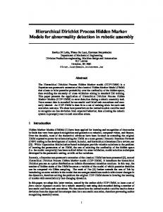
End if Until = Example: The classes Ci ; i  1,...,5 shown in Fig. 1, construct three levels L0 , L1 and L2 , the class C1 which is situated in the level L1 , is closed by way of contribution of the level L 2 .

In this section, we consider HMM, Let G=(S, U) be the graph associated with the HMM, that is, the state space S represents the set of nodes and U  {(i, j )  S 2 : aij  0} the set of directed arcs. 1) Decomposition into levels The state space can be partitioned into strongly connected classes C1 , C2 ,..., CH . Note that the strongly connected classes are defined to be the classes with respect to the relation on G defined by: i is strongly connected to j if and only if i=j or there exist a directed path from i to j and directed path from j to i. There are many good algorithms in graph theory for the computations of such partition, see [15]. Now we construct by induction the levels of the graph G. The level L0 is formed by all classes Ci such that Ci is closed, that is, any arc emanating from Ci has both nodes in Ci . The path level L p is formed by all classes Ci such that the end of any arc emanating from Ci is in some level Lp 1 , Lp 2 ,..., L0 . Remark 4.1. Let Ci be strongly connected class in the level L p then Ci is closed with respect to the restricted HMM to the state space S  ( Lp 1, Lp  2 ,..., L0 ) . It is clear that, from Remark 4.1, the following algorithm finds the levels Algorithm 4.1.

Beginning

S p0

Fig. 1.

Construction of levels

2) Restricted HMM for decoding problem using Forward algorithm In what follows, we construct, by induction, the restricted HMMs corresponding to each level Lp ; p  n,...,0 .Let ( C pk ) ,

k {1, 2,..., K ( p)} be the K th strongly connected class corresponding to the nodes in level p, where K(p) represent the maximum of the classes included in the level p. a) Construction of the restricted HMM in level Ln

12 | P a g e www.ijacsa.thesai.org

IJACSA Special Issue on Selected Papers from Third international symposium on Automatic Amazigh processing (SITACAM’ 13)

For each k  1, 2, K  n  , we denote by HMM nk the restricted HMM corresponding to the class Cnk that is the restricted HMM in which the state space restricted is Snk  Cnk ; the same M symbols O1 , O2 ,..., OM ; the matrix of transition probabilities and the matrix of observation probability are restricted to Snk .

1, pk (i)   i  bi (o1 ) if i  C pk

1, pk (i)  1,mk ' (i) if i   (C pk ), (i  Cmk ' , m  p) Step2 : Iteration t  1, T  1 ,

For

  t 1, pk ( j )    t , pk (i)  aij  b j (ot 1 ) if j  C pk i  S  (11) t 1, pk ( j )  t 1,mk ' ( j ) if j   1 (C pk ), ( j  Cmk ' , m  p)

For each k  1, 2, K  p  and p  n  1,...,0 we denote by HMM pk the restricted HMM corresponding to the class C pk .

pk

Step2 : Termination

Let 1 (C pk ) be the set of predecessors for each state i  C pk .The restricted HMM pk defined by:

P(O |  ) 

The state space: S pk  C pk  1 (C pk ) . where aij  Ppk ( j | i) if j  C pk .

The same symbols O  O1, O2 ,..., OM  . The probability distribution of the initial    i iC , where  (i)  P(s1  Si ) if i  Cpk .

state

pk

The matrix of observation probability B  b j (m)  , jC pk

where bj (m)  P(ot  Om | st  S j ) if j  C pk . V. We

denote

IMPROVED FORWARD ALGORITHM

t , pk (i), t {1,...,T}, p=n,...,0 and

by

k={1,..,K(p)} the Forward variable in state i  C pk . Lemma 5.1. Let j  C pk , the Forward variable for j at time t+1 is defined by: 

t 1, pk ( j )  



i  S pk



t , pk (i)  aij  b j (ot 1 ) 

VI.

(9)

P( xt  j | xt 1  i)  0 ,  j  C pk , these states belongs to the original set states of the class C pk or i  1 (C pk ) .

T , pk (i)

(12)

COMPLEXITY

The classical Forward algorithm generate N (N +1) (T-1) + N multiplication and N (N-1) (T-1) addition, it takes on the order of N 2T computations, which represents the quadratic complexity in the number of state. Whereas, the complexity of improved Forward algorithm can be calculated by using Akra Bazzi theorem [16] (A generalization to the well known Master Theorem [17]) which allows calculating the complexity for this type of problem. Therefore, it will be quasi-linear, equal to N log( N ) . VII. CONCLUSION The Forward algorithm progressively calculate the probability of an observation sequence, it is used in the recognition and learning because it represents the basis for revaluation in the Baum-Welch algorithm. We benefited from the method divide and conquer to reduce the charge of calculation of the Forward algorithm. [1]

Proof. From equation (7) to calculate the Forward variable t 1 ( j ) we need only the states i such as

[2] [3]

[4]

Remark 5.1. To calculate the Forward variable t 1, pk ( j ) we

[5]

need the Forward variable t , pk (i) for each i  1 (C pk ) , therefore, we always need some values that have been already calculated in the upper levels.

[6]

Algorithm 5.1.

[7]

Step1 : Initialization

n K ( p)

 

p  0 k 1 i  C pk

The matrix of transition probabilities A: for each j, i  S pk , iS pk

p=n,...,0 and k  1, 2,K  p  ; let

j  S pk

b) Construction of the restricted HMM in level Lp , p  n  1,...,0

A=  aij 

(10)

1

REFERENCES Pellegrini T., Duée R., “Suivi de Voix Parlée grace aux Modèles de Markov Cachés,” IRCAM, PARIS, 2003. Juang B. H., Rabiner L. R., “Hidden Markov Models for Speech Recognition,” Technometrics, Vol. 33, No. 3. 1991, pp. 251-272. Ramy Al-Hajj M., Chafic Mokbel, Laurence Likforman-Sulem, “Reconnaissance de l’écriture arabe cursive: combinaison de classifieurs MMCs à fenêtres orientées,” Université de Balamand, Faculté de Génie, 2006, pp 1-6. Ben Amara N., Belaïd A., Ellouze N., “Utilisation des modèles markoviens en reconnaissance de l'écriture arabe état de l'art,” Colloque International Francophone sur l'Ecrit et le Document (CIFED'00), Lyon, France. Nakai M., Akira N., Shimodaira H., Sagayama S., “Substroke Approach to HMM-based On-line Kanji Handwriting Recognition,” Sixth International Conference on Document Analysis and Recognition (ICDAR 2001), pp.491-495. Krogh A., I.Saira Mian, Haussler D., “A hidden Markov model that finds genes in E.coli DNA,” Nucleic Acids Research, Vol. 22, No. 22. Morwal S., Jahan N., Chopra D., “Named Entity Recognition using Hidden Markov Model (HMM),” International Journal on Natural Language Computing (IJNLC), 2012, Vol. 1, No.4.

For p=n,...,0 and k  1, 2,K  p  ; let i  S pk

13 | P a g e www.ijacsa.thesai.org

IJACSA Special Issue on Selected Papers from Third international symposium on Automatic Amazigh processing (SITACAM’ 13) Rabiner R., “A tutorial on Hidden Markov Models and Selected Applications in Speech Recognition,” Proceding of the IEEE, Vol. 77, No. 2. 2010. [9] Dequier J., “Chaînes de Markov et applications,” Centre D'enseignement de Grenoble, 2005, pp.9-35. [10] Khreich W., Granger E., Miri A., Sabourin R., “On the memory complexity of the forward–backward algorithm,” Pattern Recognition Letters 31. 2010. [11] Rust J., “Using Randomization to Break the Curse of Dimensionality,” Econometrica, Vol. 65, No. 3, May, 1997, pp. 487-516. [12] Van Caneghem M., “Algorithmes recursifs Diviser pour régner,”, 2003. [8]

[13] Canet L., “Algorithmique, graphes et programmation dynamique,” 2003, pp 23-25. [14] Cherki D., “decomposition des problemes de decision markoviens,” Thesis of doctorat in Faculty of science Rabat, 2002, pp 64-69. [15] Gondran M., Minoux M., “Graphes et Algorithmes” 2 nd edition, 1990. [16] Drmota M., Szpankowski W., “A Master Theorem for Discrete Divide and Conquer Recurrences,” Austrian Science Foundation FWF Grant No. S9604. [17] Roura S. (March 2001), “Improved Master Theorems for Divide-andConquer Recurrences,” Journal of the ACM, Vol. 48, No. 2, pp. 170– 205.

14 | P a g e www.ijacsa.thesai.org