estimation of poverty and income distribution related parameters in small geographic ..... It is different from the zero-inflated model considered in Wiezcorec et al.
Hierarchical Beta regression models for the estimation of poverty and inequality parameters in small areas Enrico Fabrizi 1 Maria Rosaria Ferrante Carlo Trivisano
2
SurveyConf2015
Berlin, 10/02/2015
1 2
Universit` a Cattolica del S. Cuore, Piacenza, Italy Universit` a di Bologna, Italy E. Fabrizi (Unicatt)
Berlin, 10/02/2015
1/1
Introduction
Outline Introduction to small area estimation; (mixed) Beta regression applied to small area estimation; estimation of the Gini concentration concentration coefficient; estimation of the poverty rate (headcount ratio);
Multivariate Beta regression applied to small area estimation. Presentation will be based on an empirical application: estimation of poverty and income distribution related parameters in small geographic regions using Italian data from EU-SILC survey Focus wrt to small area literature we focus on area level modelling our approach to estimation is Bayesian. Relevant posterior distribution approximated by means of MCMC algorithms. E. Fabrizi (Unicatt)
Berlin, 10/02/2015
2/1
Introduction
Small area estimation Large social sample surveys, such as the EU-SILC are designed to provide estimates of indicators for whole countries or regions, social groups within countries; Most of these measures are often needed for a collection of geographically small areas, as indicators may be distributed unevenly among the subsets of relatively small regions; For these small areas the available samples are not large enough to allow the ordinary survey sampling estimators to be precise enough; Small area estimation studies how to obtain reliable estimates in these situations; The basic idea is that of complementing survey sample information with information from other sources.
E. Fabrizi (Unicatt)
Berlin, 10/02/2015
3/1
Introduction
Motivating Example: estimating poverty parameters in health districts We have been asked to estimate several poverty related parameters the at-risk-of-poverty rate, the Gini coefficient, the relative median at-risk-of-poverty gap, material deprivation rates,
for the health districts of the administrative region Emilia-Romagna and Tuscany. Health districts play a key role in the implementation of social and health expenditure programmes aimed at the contrast of social exclusion in Italy. Auxiliary information available for each area include average taxable income claimed by private residents, perc. of residents filling tax forms, dependency ratio, percentage of resident immigrants. E. Fabrizi (Unicatt)
Berlin, 10/02/2015
4/1
Introduction
Definitions We use data from the EU-SILC sample survey (2010 wave); The at-risk-of-poverty rate, mean poverty gap, the Gini coefficient are all based on the distribution of equivalized disposable income: eq.income =
total disposable household income equivalized household size
Note that the equivalized disposable income is the same for all members of an household (i.e. we do assume 0 inequality within households); Material deprivation rates are based on a battery of nine 0/1 questions, simply counting the ‘ones’ as a rough measure of poverty severity at the household level.
E. Fabrizi (Unicatt)
Berlin, 10/02/2015
5/1
Introduction
Choices
For illustrative purposes we focus on the Gini coefficient, the at-risk-of-poverty rate There exist several approaches to small area estimation. In this presentation we focus on area level modelling The approach we adopt to estimation is Bayesian, with relevant posterior distributions approximated by means of MCMC methods.
E. Fabrizi (Unicatt)
Berlin, 10/02/2015
6/1
Introduction
Small area estimation: area level approach The area-level approach is based on the idea of complemeting survey-weighted estimators with auxiliary information accurately known at the area level through the use of models; Fay-Herriot type of models are popular: � � θˆd ∼ D1 [θd ], [Vd ] � � f (θd ) ∼ D2 [xtd β], [A] where i = 1, . . . , m ranges over the set of the target areas. In the original formulation D1 ≡ D2 ≡ N (., .), f ≡ I(.) but alternative assumptions are also possible; The (approximate) unbiasedeness of θˆd is assumed. E. Fabrizi (Unicatt)
Berlin, 10/02/2015
7/1
Beta regression in SAE
Beta regression applied to small area estimation The parameters we consider, as many others that describe poverty, social exclusion and inequality have the (0, 1) interval as support; Beta regression models represent a popular solution in this case. In the Beta distribution expected value and variance depend on both parameters Models based on Beta distributions not a straightforward extentions of Normal models. Multivariate small area models can be useful to improve precision of small area parameters estimators as they allow for borrowing strength across parameters No easy generalization of Betas to the multivariate case. E. Fabrizi (Unicatt)
Berlin, 10/02/2015
8/1
Gini coefficient
Univariate Beta regression - 1 Estimating the Gini concentration coefficient of equivalized disposable household income in health districts
E. Fabrizi (Unicatt)
Berlin, 10/02/2015
9/1
Gini coefficient
Gini concentration coefficient Popular inequality measure, often used in the economic debate; It can be defined as Z 1 Z γ=2 (y − L(y))dy = 1 − 2 0
0
1
L(y)dy =
1 ∆ 2µ
where Y is a (positive) Z ysize variable, F (y) the CDF and f (y) the −1 density, L(y) = µ F −1 (t)dt with µ = E(Y ) the Lorenz curve, 0
∆ the absolute mean difference. In the Laeken indicators framework it measures inequality among individual incomes, although all individuals within an household share the same equivalized income
E. Fabrizi (Unicatt)
Berlin, 10/02/2015
10 / 1
Gini coefficient
Estimating the Gini coefficient from survey data Survey weighted estimator 1 gd = 2Yˆ¯d
Pnd Pnd j=1
k=1 wdj wdk |ydj ˆ2 N d
− ydk |
ˆd = Pnd wdj , where N j=1 ˆ −1 Pnd wdj ydj . Yˆ¯d = N d
j=1
Pre-processing of data Many papers on Pareto tail modelling, but few consider the complex samples context; We follow Alfons et al. (2013) and replace tail observations with data generated from a Pareto; threshold estimation based on Van Kerm’s method, shape parameter on partial density components. E. Fabrizi (Unicatt)
Berlin, 10/02/2015
11 / 1
Gini coefficient
Properties of gd in small samples: problems
severe negative bias. Under SRS B(gd ) = O(n−1 ) (Deltas, 2003; Davidson, 2009); the MSE gd becomes unacceptably large; positively skewed sampling distribution; sensitivity to outliers. We proceed in two steps: propose a modified direct estimator (with smaller bias); model the modified estimator.
E. Fabrizi (Unicatt)
Berlin, 10/02/2015
12 / 1
Gini coefficient
A simulation study on small-sample properties of gd
We introduce a simple simulation exercise based on synthetic the data set eusilcP from the R package simFrame (Alfons et al., 2010) data are generated from the real Austrian sample of the EU-SILC survey. In the MC experiment, we draw stratified cluster random sampling from the 9 federal states sub-samples, using households as clusters. The overall sample size in terms of households m = 130 is allocated to strata almost proportionally. We generated sample weights incorrelated with income, with variance and skeweness matching those of our actual sample.
E. Fabrizi (Unicatt)
Berlin, 10/02/2015
13 / 1
Gini coefficient
Simulation results Area Burgenland Vorarlberg Salzburg Carinthia Tyrol Styria Upper Austria Lower Austria Vienna
md 4 6 8 10 12 15 20 25 30
γd 25.09 27.85 31.71 26.44 25.18 25.82 25.55 25.05 29.68
rbias(gd ) -0.33 -0.24 -0.19 -0.16 -0.12 -0.12 -0.08 -0.06 -0.06
rbias(gd ) = B(gd )/γd , rrmse(gd ) =
p
rrmse(gd ) 0.49 0.37 0.35 0.32 0.31 0.26 0.24 0.23 0.18
M SE(gd )/γd ;
We also studied the distribution of the squared income (higher concentration). The size of the relative bias is larger.
E. Fabrizi (Unicatt)
Berlin, 10/02/2015
14 / 1
Gini coefficient
Reducing the bias of the direct estimator
The assumption E(θˆd |θd ) ∼ = θd fails. We introduced the modified estimator Pnd Pnd 1 j=1 k=1 wdj wdk |ydj − ydk | g˜d = ˆ 2 − Pmd w N ˜2 2Yˆ¯ d
2 = where w ˜dh
d
h=1
dh
Pnh
j=1 wdj .
Under SRS this amounts to replace n2 with n(n − 1) under SRS (see Jasso, 1978; Deltas, 2003); the remaining bias is of smaller order (with unpredictable sign).
E. Fabrizi (Unicatt)
Berlin, 10/02/2015
15 / 1
Gini coefficient
Back to simulation results
Area Burgenland Vorarlberg Salzburg Carinthia Tyrol Styria Upper Austria Lower Austria Vienna
E. Fabrizi (Unicatt)
γd 4 6 8 10 12 15 20 25 30
md 25.09 27.85 31.71 26.44 25.18 25.82 25.55 25.05 29.68
rbias(gd ) -0.33 -0.24 -0.19 -0.16 -0.12 -0.12 -0.08 -0.06 -0.06
rrmse(gd ) 0.49 0.37 0.35 0.32 0.31 0.26 0.24 0.23 0.18
rbias(˜ gd ) 0.01 0.00 -0.01 -0.01 0.01 -0.02 0.01 0.01 -0.01
rrmse(˜ gd ) 0.53 0.37 0.35 0.32 0.32 0.25 0.25 0.24 0.18
Berlin, 10/02/2015
16 / 1
Gini coefficient
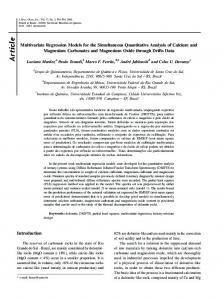
A Beta regression model for the Gini coefficient ! 2φgd 2φgd − γd (1 + γd ) 1 − γd g˜d ∼ Beta − γd , , 1 + γd 1 + γd γd that implies E(˜ gd |γd , φgd ) = γd V (˜ gd |γd , φgd ) = (2φgd )−1 {γd2 (1 − γd2 )}
0.00
0.05
0.10
y
0.15
0.20
0.25
Variance as a function of γd :
E. Fabrizi (Unicatt)
0.0
0.2
0.4
0.6
0.8
1.0
Berlin, 10/02/2015
17 / 1
Gini coefficient
The assumption on the variance
The expression for V (˜ gd |γd ) can be justified using different arguments: Sarno (1988) analyzes the shape of the variance of the gini coefficient under different parametric models and finds a ’negatively skewed’ shape for the variance function, largerly consistent with the one that we derived; assuming log-normality of Y and SRS it can be shown that: γ 2 (1 − γd2 ) Vsrs (˜ gd ) ∼ . = d 2nd
E. Fabrizi (Unicatt)
Berlin, 10/02/2015
18 / 1
Gini coefficient
The assumption on the variance - 2
by simulation (the same we introduced before)
0.04
●
● ●
●
0.02
γd2(1 − γd2) nd
0.03
●
● ●● ●
0.01
●
●
●●
● ● ●
● ● ● ● ● ●● ●● ● ●
0.005
0.010
0.015
Monte Carlo variances
E. Fabrizi (Unicatt)
Berlin, 10/02/2015
19 / 1
Gini coefficient
Parameter φd Assuming φd = md βφ is sensible; In principle a prior for φd could be specified and uncertainty about its estimation accounted for; Assuming (smoothed) variances of direct estimators is a standard assumption in small area literature.
We estimate φd with a variance smoothing model: g˜d2 (1 − g˜d2 ) = βφ nd + ed 2Vboot (˜ gd ) φˆd = nd βˆ The fit on our data set is very good with a R2 = 0.89 E. Fabrizi (Unicatt)
Berlin, 10/02/2015
20 / 1
Gini coefficient
Modelling Gini coefficient: structural part
logit(γd ) = xTd β γ + vd where xd contains auxiliary information for area d. ind
vd ∼ N (0, σv2 ) For the prior of the variance component we assume: σv ∼ half-t(ν = 2, A = 1) (in line with Gelman, 2006). We prefer ν = 2 instead of ν = 1 (half-Cauchy) for consistency with the multivariate priors (later). We chose A = 1 after careful consideration of the scale of the parameters’ and sensitivity analysis. E. Fabrizi (Unicatt)
Berlin, 10/02/2015
21 / 1
Gini coefficient
Modelling Gini coefficient: prior on the variance components
To specify the prior we use a redundant product parametrization that has the merit to speed up MCMC computations: p vd = vd? ζ vd? ∼ N (0, η 2 ) ζ ∼ Gamma(1/2, A−2 )
,
η 2 ∼ IGamma(ν/2, ν)
It can be shown � that: � q 1. vd |η ∼ V G 21 , η22A2 , 0, 0 ,V (vd |η) =
η 2 A2 2
2. If we define σv2 = ζη 2 then σv ∼ half-t(ν, A).
E. Fabrizi (Unicatt)
Berlin, 10/02/2015
22 / 1
Gini coefficient
Modelling Gini coefficient: alternative priors We consider two alternatives for priors on random effects: i) vd ∼ N (0, σv2 ) with σv−2 ∼ Gamma(a, b); ii) vd ∼ t(0, κ, σv2 ) with κ ∼ Exp(c) and σv−2 ∼ Gamma(a, b). We use ordinary model selection tools, specifically the Deviance Information Criterion (DIC) and the logarithm of the pseudo-marginal likelihood (LPLM). Efficiency improvements are measured by: s V (γd |data) SDR(γd ) = 1 − E[V (˜ gd |γd )|data]
E. Fabrizi (Unicatt)
Berlin, 10/02/2015
23 / 1
Gini coefficient
Gini coefficient: empirical results
Model selection for alternative prior specifications on the random effects and the variance component (v.c.): prior on vd N (0, σv2 ) N (0, σv2 ) t(0, κ, σv2 )
prior on v.c. σv ∼ half-t(ν = 3, A = 1) σv−2 ∼ Gamma(0.01, 0.01) σv−2 ∼ Gamma(0.01, 0.01)
E. Fabrizi (Unicatt)
DIC -221.7 -222.2 -222.0
LP LM 111.5 111.2 111.1
ASDR 0.623 0.523 0.516
Berlin, 10/02/2015
24 / 1
Gini coefficient
1.0
0.40
Gini coefficient: empirical results
0.8
0.35
●
● ●
● ●
● ● ●
E(γd | data)
● ●
● ● ●
0.25
●
●
●
● ●
●
● ● ● ● ●● ● ● ● ●● ● ● ● ●●● ● ● ● ● ●● ● ● ● ● ● ●
● ● ●
● ● ●
●
0.6
●
●
●
● ●
● ● ● ●
● ● ● ● ● ● ● ● ● ●
SDR(γd)
●
●
●
● ●
●● ● ●
● ● ●
●
●
●
●
●
●
●
● ●
● ●
●
●
●
●
● ● ●
● ●
●●
●
●
● ● ● ● ●● ●
0.4
0.30
●
● ●
● ●
● ● ● ●
0.0
0.15
0.2
0.20
●
0.15
0.20
0.25
0.30 ~ gd
E. Fabrizi (Unicatt)
0.35
0.40
0
20
40
60
80
100
120
md
Berlin, 10/02/2015
25 / 1
Poverty rate
Univariate Beta regression - 2 Estimating the at-risk-of-poverty rate in health districts
E. Fabrizi (Unicatt)
Berlin, 10/02/2015
26 / 1
Poverty rate
Targeting the at-risk-of-poverty rates: basic model Direct survey-weighted estimator pd approximately unbiased in this case: E(pd ) ∼ = πd Standard area-level model for proportions: � � pd |πd , φd ∼ Beta πd (φd − 1), (1 − πd )(φd − 1) that implies E(pd |πd , φd ) = πd , V (pd |πd , φd ) = φ−1 d {πd (1 − πd )} φd can be interpreted as a SRS-equivalent sample size for the actual design. It can be estimated using boostrap + variance smoothing function. E. Fabrizi (Unicatt)
Berlin, 10/02/2015
27 / 1
Poverty rate
At-risk-of-poverty rates: the problem of pd = 0 estimates
The problem pd has a discrete sampling distribution. pd = 0 likely to be observed, especially when πd and/or md small; pd = 1 also possible in principle (but unlikely in our problem). Assumptions Although pd = 0, we assume that πd > 0, i.e. there are no areas without poor households at the population level; Under SRS of md households with probability of being poor πd , we would have P (pd = 0|πd > 0) = (1 − πd )md
E. Fabrizi (Unicatt)
Berlin, 10/02/2015
28 / 1
Poverty rate
At-risk-of-poverty rates: zero inflated model We specify the model
pd =
0
with prob. (1 − πd? )md
Pd with prob. 1 − (1 − πd? )md
where � Pd ∼ Beta πd? (φd − 1), (1 − πd? )(φd − 1) π ? (1−π ? )
so that E(Pd |πd? ) = πd? , V (Pd |πd? ) = d φd d . Note that πd = {1 − (1 − πd? )md }πd? It is different from the zero-inflated model considered in Wiezcorec et al. (2011) where P (pd = 0) is modelled as function of covariates and not of the sample size. E. Fabrizi (Unicatt)
Berlin, 10/02/2015
29 / 1
Poverty rate
Variance smoothing Note that πd? (1 − πd? ) {1 − a(πd? )} + φd + a(πd? ){1 − a(πd? )}πd2?
V (pd |πd? ) =
(Ospina and Ferrari, 2012), a(πd? ) = (1 − πd? )md . only the first addend of V (pd |πd? ) depends on φd we estimate φd using smoothing bootstrap estimates Vˆ (pd |pd > 0). Smoothing model: pd (1 − pd ) = βf nd + ed = φˆd + ed ˆ V (pd |pd > 0)
E. Fabrizi (Unicatt)
Berlin, 10/02/2015
30 / 1
Poverty rate
Targeting the at-risk-of-poverty rates: structural part
logit(πd ) = xTd β π + vd where xd contains auxiliary information for area d. ind
vd ∼ N (0, σv2 ) For the prior we assume σv ∼ half-t(ν = 2, A = 1) (as before).
E. Fabrizi (Unicatt)
Berlin, 10/02/2015
31 / 1
Poverty rate
0.25
At-risk-of-poverty rates: empirical results
0.8
●
0.20
● ●
●
●
● ●
● ● ● ● ●
●
●●
●
●
● ● ●
● ●
● ●● ●
● ● ●
●
●
● ●● ●
●● ● ● ● ● ● ● ● ●● ●
●
●
●
● ●
●
●● ● ●
● ●●
● ●
●
●
●
●
● ●
●
0.2
●
0.05
●
● ● ●● ●● ●● ● ●
●●
●
●
SDR(πd)
● ● ●
● ●● ● ● ● ● ●
0.4
0.15
● ●
●
● ●
● ●
0.10
E(πd | data)
●
●
●
0.6
●
● ●
●
● ●● ● ●●● ● ●● ● ● ● ● ● ●
●
0.0
0.00
●
0.00
0.05
0.10
0.15
0.20
0.25
0
pd
20
40
60
80
100
120
md
Efficiency improvements are measured by: s V (πd |data) SDR(πd ) = 1 − −1 φˆ E(πd (1 − πd )|data) d
E. Fabrizi (Unicatt)
Berlin, 10/02/2015
32 / 1
Multivariate model
Multivariate Beta regression Joint estimation of the at-risk-of-poverty rate and the Gini coefficient in health districts
E. Fabrizi (Unicatt)
Berlin, 10/02/2015
33 / 1
Multivariate model
A multivariate model
We want to specify a multivariate area level model for (pd , g˜d ) to exploit their correlation (both are functions of equivalized income) Challenges No simple multivariate generalizations of the Beta distribution with flexible correlation structure; pd is a 0-mixture of Betas; This motivates our recours to copula functions. Specifically, we propose the use of Gaussian copulas (a special case of inversion copulas parametrized by a correlation matrix R).
E. Fabrizi (Unicatt)
Berlin, 10/02/2015
34 / 1
Multivariate model
Gaussian copula functions
f (x1 , . . . , xk ) =
g(x1 ) × · · · × g(xk ) 1
|R| 2
exp
n
o 1 − zTk (R−1 − Ik )zk 2
where zTk = (Φ−1 {G1 (x1 )}, . . . , Φ−1 {Gd (xk )}, Gi (xi ) the CDF of Xi (density gi (xi )). Here X1 = pd , X2 = g˜d , k = 2. We calculate R using correlations between direct estimators (pd , g˜d ) according to the following steps: 1
Calculate Spearman rank empirical correlation between pd , g˜d using bootstrap (ρˆ¯boot );
2
average correlations over the set of the largest domain (largest half);
3
monotone transformation of correlations;
4
product correlation obtained by means of r = 2 sin(π ρˆ¯boot ). E. Fabrizi (Unicatt)
Berlin, 10/02/2015
35 / 1
Multivariate model
Multivariate model: structural part Let logit(πd ) = ξ1d , logit(γd ) = ξ2d , ξ d = (ξ1d , ξ2d )T . We assume ξ d ∼ M V N (ν d , Σb ) with ν1d = xti β ν1 , ν2d = xti β ν2 This specification assumes correlation between underlying population parameters. Diffuse normal priors are assumed for β ν1 and β ν2 . For Σa we follow the suggestion of Huang and Wand (2013): � −1 Σb |a1 , a2 ∼ Inv-Wishart ν + 1, 2νdiag(b−1 1 , b2 ) �1 1 � bi ∼ Inv-Gamma , 2 , i = 1, 2. 2 Bi This prior marginally induces σi ∼ half − t(ν, Bi ). We set B1 = B2 = 1. ν = 2 that induces a marginal uniform prior for the correlation between the two random effects. E. Fabrizi (Unicatt)
Berlin, 10/02/2015
36 / 1
Multivariate model
Multivariate model: results Model comparison using DIC (and the measure of model complexity pD): Model uu um mm
DIC -353.3 -361.2 -370.9
pD 43.91 51.03 41.66
uu = univariate model; um = assumes cor(pd , g˜d ) = 0, but allows correlation between parameters; mm = multivariate model. mm is best also in terms efficiency improvements. Same sorting of models if we consider theP log of the pseudo-maximumu-likelihood: LP LM = m d=1 log(CP Oi ).
E. Fabrizi (Unicatt)
Berlin, 10/02/2015
37 / 1
Multivariate model
0.050
0.20
Univariate and multivariate models for πd
0.045
●
● ●
●
●
● ● ●
● ● ● ● ● ● ● ● ●● ● ●● ●●
●
0.05
0.10
0.15
E(πd | data) univariate model
0.20
● ●
● ●
● ●
●
0.015
● ● ● ●
0.05
● ●
0.020
● ● ● ●●●● ●● ● ●● ● ● ●
● ●
0.035
●
0.030
sd(πd | data) multivariate model
● ●● ● ● ●● ●● ● ● ●● ● ●
0.025
0.15
●
●
●
0.10
E(πd | data) multivariate model
●
0.040
●●
●
●
●
●
●
● ●
● ● ● ●● ● ● ●● ● ● ●
● ● ●● ● ●●● ●● ●● ● ● ● ● ● ● ● ●
●
● ● ● ● ● ● ● ● ● ●
●
0.015
0.020
0.025
0.030
0.035
0.040
0.045
0.050
sd(πd | data) univariate model
the two sets of direct estimates are largely consistent with a slightly more pronounced shrinkage effect for the multivariate model; There is an efficiency improvement effect when passing from univariate to multivariate modeling. On average SDR goes from 0.53 to 0.57. E. Fabrizi (Unicatt)
Berlin, 10/02/2015
38 / 1
Multivariate model
Software Posterior distributions are approximated by MCMC methods using the OpenBugs software. Remarks 1 Beta mixture density requires the use of ‘tricks’ (explicit writing of the log-likelihood); 2 In programming copulas: we empirically calculated the CDF from the Markov Chains using the cumulative function; Φ−1 (.) (available only as link in Openbugs) is approximated using the solver solution 3
Multivariate priors for variance components are programmed using an extension of parameter expansion representation proposed by Gelman (2006) for the half-t.
All codes are available upon request from the authors (and will be published). E. Fabrizi (Unicatt)
Berlin, 10/02/2015
39 / 1
Multivariate model
Conclusions
We apply Bayesian Beta regression modeling to small area Fay-Herriot type of models for poverty and inequality related parameters, focusing on specific problems: parametrizations consistent with realistic variance smoothing models; accomodation of direct estimates equal to 0 (or 1); introduction of flexible multivariate models based on Gaussian copula functions. The presented material is part of a wider research that include also multivariate Beta modeling of poverty rates based on increasing thresholds (or other groups of increasing sortable parameters with support (0,1))
E. Fabrizi (Unicatt)
Berlin, 10/02/2015
40 / 1
References
References Alfons A., Templ M., Filzmoser P. (2013), Robust estimation of economic indicators from survey samples based on Pareto tail modeling, Journal of the Royal Statistical Society, ser. C, 62, 271–286. Griffin J.E., BrownP.J. (2010) Inference with normal-gamma prior distributions in regerssion problems, Bayesian Analysis, 5, 171–188; Davidson R. (2009), Reliable inference for the Gini index, Journal of Econometrics, 150, 30-40. Huang A., Wand M.P. (2013), Simple marginally noninformative prior distributions for covariance matrices, Bayesian Analysis, 8, 439-452; Ospina R., Ferrari S.L.P. (2012), A general class of zero-or-one inflated beta regression models, Computational Statistics and Data Analysis, 56, 1609-1623; Wieczorek J., Hawala S. (2011), A Bayesian zero-one inflated Beta model for estimating poverty in U.S. counties, JSM Proceedings, Section on Survey Research Methods, 2812-2822. E. Fabrizi (Unicatt)
Berlin, 10/02/2015
41 / 1
References
References
The presentation is based on E. Fabrizi, M.R. Ferrante, C. Trivisano (2016) Hierarchical Beta regression models for the estimation of poverty and inequality parameters in small areas, in: Pratesi, Monica (Ed.): Analysis of poverty data by small area methods. John Wiley and Sons, pp 299-314).
E. Fabrizi (Unicatt)
Berlin, 10/02/2015
42 / 1