Hierarchical Clustering with Concave Data Sets

Metodološki zvezki, Vol. 2, No. 2, 2005, 173-193

Hierarchical Clustering with Concave Data Sets Matej Francetič, Mateja Nagode, and Bojan Nastav1

Abstract Clustering methods are among the most widely used methods in multivariate analysis. Two main groups of clustering methods can be distinguished: hierarchical and non-hierarchical. Due to the nature of the problem examined, this paper focuses on hierarchical methods such as the nearest neighbour, the furthest neighbour, Ward’s method, between-groups linkage, within-groups linkage, centroid and median clustering. The goal is to assess the performance of different clustering methods when using concave sets of data, and also to figure out in which types of different data structures can these methods reveal and correctly assign group membership. The simulations were run in a two- and threedimensional space. Using different standard deviations of points around the skeleton further modified each of the two original shapes. In this manner various shapes of sets with different inter-cluster distances were generated. Generating the data sets provides the essential knowledge of cluster membership for comparing the clustering methods’ performances. Conclusions are important and interesting since real life data seldom follow the simple convex-shaped structure, but need further work, such as the bootstrap application, the inclusion of the dendrogram-based analysis or other data structures. Therefore this paper can serve as a basis for further study of hierarchical clustering performance with concave sets.

1

Introduction

Clustering methods represent one of the most widely used multivariate techniques in practice. Essentially, there are two main groups of these methods: hierarchical and non-hierarchical. Statistics mainly uses the latter; this paper, on the other hand, primarily deals only with hierarchical clustering methods. The idea behind this decision is that the non-hierarchical methods, the most widely used being the k-means method, do not perform well with concave sets of data, since the centroids’ usage results in wrong classifications. Although several hierarchical clustering methods exist this paper focuses on the methods implemented in the statistical software SPSS. These are: the nearest neighbour, the furthest neighbour, centroid 1

University of Ljubljana, Slovenia

174

Matej Francetič, Mateja Nagode, and Bojan Nastav

method, median clustering, linkage between groups and within linkage groups, and Ward’s method. Due to high discrepancies in naming the methods, we will follow the SPSS wording. The primary aim of this paper is to assess the performance of different clustering methods when using concave sets of data and also to figure out in which types of different data structures these methods can reveal and correctly assign group membership. Sets of points differing in shape (skeleton) and inter-point distance were used in the analysis: the simulations were run in a two and threedimensional space with different standard deviations of points around the skeleton. Generating the sets of points gave an advantage, since the knowledge of cluster membership is essential in comparing the performances of clustering methods (perhaps better “in comparing”). In this manner various shapes of sets with different inter-cluster distances were generated. Certain limitations were imposed since the used parameters can lead to a vast number of generated sets. Applying different hierarchical clustering methods to these generated sets was the basis for assessing clustering accuracy and by this the performance of different hierarchical clustering methods for concave sets of data. We have not come across any studies dealing with hierarchical clustering on concave data; the latter are however, mainly dealt with other, “modern” methods, such as the fuzzy or wave clustering (see section five). The paper consists of two parts. First we introduce the research methodology and briefly outline the methods used (section two). In the second part, a report of generating data sets is presented in section three and presentation of the results of successfulness of different clustering methods performed on the generated data in section four. Section five concludes the work and presents suggestions for possible further research.

2

Clustering

Clustering is believed to be one of the mental activities that human beings have been using for centuries. Classifying objects into classes has improved the control over objects classified and deepened the understanding of different classes. Gathering and accumulation of knowledge would be of no practical use without clustering (perhaps better “without clustering”). Besides the spread of knowledge base time has also brought an advance in clustering methods. Nowadays, despite the mathematical and statistical primacy over the methods, other fields, especially medicine and marketing, find clustering as a very useful tool. The goal of clustering is to merge objects (units or variables) with regard to their characteristics and, by doing so, obtain internal homogeneity and external heterogeneity (isolation) of classes (clusters) produced. Characteristics, or better, the criteria according to which the objects are clustered, are usually, depending on the method used, based on the proximity matrix, which measures the objects’

Hierarchical Clustering With Concave Data Sets

175

distances or similarities. Our work was based on hierarchical clustering in SPSS (see description of methods below) and distance was the tool used for measuring the similarity among objects. To be more precise, we have used Euclidian distance, which can be presented by the following equation (or graphically presented in Figure 1):

 p Dij =  ∑ X ik − X jk  k =1 

2

   

1/ 2

(2.1)

Figure 1: Euclidian distance for two points A and B.

Euclidian distance measures the actual (spatial) distance between two objects (Figure 1 gives a presentation of two-dimensional space, but can be applied to p variables using Equation (2.1)). Other distances could be used as well, such as Mahalonobis distance, which is a statistical distance (taking into account the standardization of units) between two points and includes covariances or correlations between variables (Sharma, 1996: 44). Applying this distance to our concave data sets would blur the picture: data would be “stretched” along some line in space and due to interlaced data its use would not lead to better results. The data used were generated (see chapter three) with no additional standardization and the Euclidian distance was applied. Choosing the tool to measure the distance is the first step. The second step is defined by the method and refers to the way this tool (distance) is applied among objects.

2.1

Hierarchical clustering

Hierarchical clustering is an iterative procedure for clustering objects. The starting point of hierarchical cluster analysis is a data matrix containing proximities between separate objects. At each hierarchical step, the two objects that are most similar, given certain criteria, depending on the method applied, are joined. A

Matej Franceti č, Mateja Nagode, and Bojan Nastav

176

joined pair is again called an object or a cluster. This means that at any hierarchical step (1) two single items may be clustered to form one new cluster, (2) a single item may be added to an existing cluster of items, or (3) two clusters may be combined into a single larger cluster. This process continues until all items are joined into only one cluster (Abswoude et al, 2004:337)

2.1.1 Nearest neighbour2 The nearest neighbour method measures distance between clusters as the distance between two points in the clusters nearest to each other. It tends to cause clusters to merge, even when they are naturally distinct, as long as proximity between their outliers is short (Wolfson et al, 2004: 610). The effect of the algorithm that it tends to merge clusters is sometimes undesirable because it prevents the detection of clusters that are not well separated. On the other hand, the criteria might be useful to detect outliers in the data set (Mucha and Sofyan, 2003). This method turns out to be unsuitable when the clusters are not clearly separated but it is very useful when detecting chaining structured data (chaining effect).

2.1.2 Furthest neighbour3 This method proceeds like the nearest neighbour method except that at the crucial step of revising the distance matrix, the maximum instead of the minimum distance is used to look for the new item (Mucha and Sofyan, 2003). That means that this method measures the distance between clusters through the distance between the two points in the clusters furthest from one another. Furthest neighbour results in separate clusters, even if the clusters fit together naturally, by maintaining clusters where outliers are far apart (Wolfson et al, 2004: 610). This method tends to produce very tight clusters of similar cases.

2.1.3 Centroid method The centroid is defined as the centre of a cloud of points (Joining Clusters: Clustering Algorithms). Centroid linkage techniques attempt to determine the ‘centre’ of the cluster. One issue is that the centre will move as clusters are merged. As a result, the distance between merged clusters may actually decrease between steps, making the analysis of results problematic. This is not the issue with single and complete linkage methods (Wolfson et al, 2004: 610). A problem with the centroid method is that some switching and reversal may take place, for 2 3

Also called Single Linkage Method or Minimum Distance Method. Also called Complete Linkage or Maximum Distance Method.


177

example as the agglomeration proceeds some cases may need to be switched from their original clusters (Joining Clusters: Clustering Algorithms).

2.1.4 Median method This method is similar to the previous one. If the sizes of two groups are very different, then the centroid of the new group will be very close to that of the larger group and may remain within that group. This is the disadvantage of the centroid method. For that reason, Gover (1967) suggests an alternative strategy, called the median method, because this method could be made suitable for both similarity and distance measures (Mucha and Sofyan, 2003). This method takes into consideration the size of a cluster, rather than a simple mean (Schnittker, 2000: 3).

2.1.5 Linkage between groups4 The distance between two clusters is calculated as the average distance between all pairs of objects in the two different clusters. This method is also very efficient when the objects form naturally distinct ‘clumps’, however, it performs equally well with elongated, ‘chain’ type clusters (Cluster Analysis).

2.1.6 Linkage within groups5 This method is identical to the previous one, except that in the computations the size of the respective clusters (i.e. the number of objects contained in them) is used as a weight. Thus, this method should be used when the cluster sizes are suspected to be greatly uneven (Cluster Analysis).

2.1.7 Ward's method The main difference between this method and the linkage methods is in the unification procedure. This method does not join groups with the smallest distance, but it rather joins groups that do not increase a given measure of heterogeneity by too much. The aim of Ward’s method is to unify the groups such that variation inside these groups does not increase too drastically. This results in clusters that are as homogenous as possible (Mucha and Sofyan, 2003). Ward’s method is based on the sum-of-squares approach and tends to create clusters of similar size. The only method to rely on analysis of variance, its underlying basis 4 5

Unweighted Pair-Groups Method Average (UPGMA). Weighted Pair-Groups Method Average (WPGMA).

Matej Franceti č, Mateja Nagode, and Bojan Nastav

178

is closer to regression analysis than the other methods. It tends to produce clearly defined clusters (Wolfson et al, 2004: 610).

3

Data generation

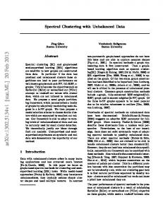
The analysis is based on concave sets of points. For the purposes of this paper the data are generated in two and three-dimensional space, however, it is easy to extend this process to a more dimensional space. This process consists of three steps. The first step is the construction of the skeleton. The skeleton is an arbitrary curve in a more dimensional space. The curve is represented as the finite set of ordered points. The points that lie on the curve between these selected points can be approximated with linear or cubic interpolation.

(a)

(b)

Figure 2: Linear (a) and cubic (b) interpolation.

The use of linear interpolation in this paper is due to simplification of the calculations that are needed for further analysis. A better approximation of the target curve can also be achieved with a larger set of ordered points.

(a)

(b)

Figure 3: Chosen points before (a) and after (b) shifting.


179

The second step is choosing the sample points. In order to do this we have normalized the length of the curve so that an arbitrary point on the curve is given by S(t), where 0