Hierarchical Error-Driven Approximation of Implicit Surfaces from ...

Eurographics Symposium on Geometry Processing (2006) Konrad Polthier, Alla Sheffer (Editors)

Hierarchical Error-Driven Approximation of Implicit Surfaces from Polygonal Meshes Takashi Kanai1 1 The

Yutaka Ohtake2

Kiwamu Kase2

University of Tokyo, Graduate School of Arts and Sciences, Japan 2 RIKEN, VCAD Modeling Team, Japan

Abstract This paper describes an efficient method for the hierarchical approximation of implicit surfaces from polygonal meshes. A novel error function between a polygonal mesh and an implicit surface is proposed. This error function is defined so as to be scale-independent from its global behavior as well as to be area-sensitive on local regions. An implicit surface tightly-fitted to polygons can be computed by the least-squares fitting method. Furthermore, this function can be represented as the quadric form, which realizes a compact representation of such an error metric. Our novel algorithm rapidly constructs a SLIM (Sparse Low-degree IMplicit) surface which is a recently developed non-conforming hierarchical implicit surface representation. Users can quickly obtain a set of implicit surfaces with arbitrary resolution according to errors from a SLIM surface. Categories and Subject Descriptors (according to ACM CCS): I.3.5 [Computer Graphics]: Curve, Surface, Solid and Object Representations, G.1.2 [Numerical Analysis]: Approximation of Surfaces and Contours

1. Introduction Polygonal mesh is nowadays recognized as a de facto standard geometric representation in the area of Computer Graphics (CG). A large variety of applications to generate or edit polygonal meshes have been developed. However, these polygonal meshes often contain defects such as gaps, T-junctions, self-intersections, and non-manifold structure. These problems must be handled with care for many purposes. Geometrically unfavorable conditions such as bad aspect ratios also render them unsuitable for other purposes such as numerical simulations. On the other hand, an implicit surface is a well-known surface representation. Geometric details of an object can be represented using less surface primitives than meshes. Since the combination of multiple implicit surfaces can define a solid model strictly, issues for meshes described above do not occur. Implicit surfaces are convenient even for geometry processing because we do not need to take into consideration the connectivity of neighbor surfaces. This paper provides a tool for rapidly converting polygonal meshes into implicit surfaces. We specifically deal with SLIM (Sparse Low-degree IMplicit) surfaces [OBA05]. Our c The Eurographics Association 2006.

algorithm can approximate a SLIM surface which has the hierarchical structure of implicit surfaces. Each node of a SLIM surface contains an error between parts of a polygonal mesh and an implicit surface which is calculated in our algorithm. It is then possible to quickly extract different resolutions of SLIM nodes according to the error specified by the user. The technical contributions of our approach include: Surface Fitting using Polygon-Implicit Error Metrics. We propose a novel error function of an implicit surface for polygons. It combines the algebraic distance and the normal error distance and is a natural extension of error functions for points. The function is also represented as a quadric form. This provides several advantages, for example, a compact storage and efficient approximation. Coefficients of an implicit function can be calculated by the least-squares fitting method. This requires only solving a small linear system. Hierarchical Implicit Surface Approximation. Our scheme for the approximation to a SLIM surface from a polygonal mesh is originated from the mesh simplification method. The algorithm itself is quite simple, fast, and robust for creating a hierarchical tree structure of

T. Kanai, Y. Ohtake & K. Kase / Hierarchical Error-Driven Approximation of Implicit Surfaces

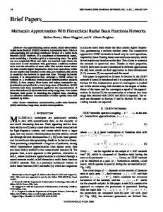
E < 1.0 × 10−1

E < 1.0 × 10−2

E < 1.0 × 10−3

E < 1.0 × 10−4

E < 1.0 × 10−5

Figure 1: Error-driven approximation of SLIM surfaces for “bimba” mesh (1.2M polygons). Different specifications of error thresholds enable us to quickly generate various resolutions of SLIM surfaces. The number of nodes is: 721, 2,258, 7,076, 22,317, and 70,273 (from left to right). Color balls shown in the bottom denote a set of supports for the corresponded SLIM surfaces. Colors are assigned according to the error E which decreases from red to green. implicit surfaces. Since our algorithm computes a set of implicit surfaces in the order of increasing errors, it is easy to build such a hierarchy based on errors. Geometric features such as creases or corners can be preserved in the process of our algorithm. Partition of Unity Evaluation with Sharp Features. To polygonize and visualize implicit surfaces with sharp features, we propose a new Partition of Unity (PU) evaluation method which can exactly estimate crease edges. This new PU method is valid for the generic representation of SLIM surfaces and is well-fitted to our approximation algorithm. Fig. 1 clearly demonstrates the characteristics of our approach. We assign an error value calculated in the approximation process to each node of a SLIM surface. Using the hierarchical structure of a SLIM surface, we can then quickly extract a set of implicit surfaces within an error threshold specified by the user. Such the run-time extraction is useful for LOD rendering of SLIM surfaces. Also, the idea of such an error-driven extraction is a natural approach to control fitting errors for the use of the applications such as CAD. 1.1. Related Work The most relevant research to ours can be seen in [SOS04]. They have proposed a construction method of implicit surfaces which approximates or interpolates polygonal meshes. Their method uses Moving Least Squares (MLS) surfaces

imposed with additional constraints such as points, normals, or integrals over polygons. The difference between their approach and ours is the algorithm of surface construction. Their algorithm first collects neighbor primitives (e.g. points, polygons) within an error threshold for each primitive. For such neighbor primitives, they fit a plane to generate a MLS surface. In contrast, our algorithm is performed hierarchically. A set of implicit surfaces with different resolutions can be generated by executing the algorithm only once. Many approaches on implicit surface reconstruction from a set of input points have been proposed. In [SPOK95, CBC∗ 01, TO02, YT02] the function is represented by globally-supported radial splines. This class of functions has a favorable property related to a solution’s global behavior. One disadvantage of these approaches is that it takes considerable time to obtain the functions. [YT02] has proposed a method to roughly match polygons by using these splines. However, the resulting implicit surfaces still deviate substantially from the input. Other types of tools for reconstruction use locallysupported implicit functions [Mur91, MYC∗ 01, OBA∗ 03, OBA05]. These approaches have the advantage that the position on a surface or its gradient can be rapidly evaluated due to their local property. Hence the local fitting scheme can be used to represent even a dense object by a large set of implicit surfaces. Our approach presented in this paper also uses this type of function. c The Eurographics Association 2006.


More recently, the implicit surface fitting scheme is utilized to obtain surface objects in some applications. [IH03] fits implicit surfaces to generate smooth 3D objects from sketch information. Basic primitives such as spheres or cylinders are locally fitted to a mesh to extract characteristic features in [WK05]. 1.2. SLIM Surfaces Our approach mainly uses SLIM (Sparse Low-degree IMplicit) surfaces [OBA05]. It is composed of hierarchical treestructured surfel nodes, each of which has low-degree implicit polynomial functions. Each surfel node is a local approximation of an object and an implicit function of a node is a rough approximation of those of its all children. A position or its gradient on a SLIM surface is represented as a blend of several wrapped neighbor surfels. MPU (Multi-level Partition of Unity) implicit surface [OBA∗ 03] is quite a similar representation to the SLIM surface. The only difference is that a hierarchical structure of a MPU surface is created by the spatial partitioning of its object. Although the original SLIM surface [OBA05] supports up to cubic degree polynomials, we use here only quadratic implicit functions for convenience. However, our approach can be applied to cubic or higher-degree polynomials. In these cases, formulae discussed in later sections are relatively complicated. 2. Implicit Quadratic Surface Fitting for Polygonal Meshes In this section, we propose a novel method to fit an implicit surface to a polygonal mesh. We indicate here a special function to measure the distance between a polygon and an implicit surface. The implicit curve or surface fitting problem has a history of over twenty years in the area of computer vision (See [Pra87] and [Tau91] for summary). One well-known function is the so called algebraic distance. It uses an absolute value of a function as an approximate distance. Although using an exact distance between a point and surface achieves better fit, it requires high computational costs because non-linear equations need to be solved [KP90]. The other function solved by linear equations is the 3L algorithm proposed in [BLCC00]. Additional points are sampled in the shrunken and expanded regions and their functional values are computed. A combined error function based on these function values is minimized by solving a linear system. [TTC00] proposed the gradient one algorithm which adds the gradient constraint of implicit curves or surfaces. [HBM04] extended an approach of [TTC00] to fit an implicit curve robustly. The difference between these error functions and ours is that our function evaluates over a polygon itself, whereas the c The Eurographics Association 2006.

others evaluate at a point set. We will show the comparison of results later in this section. In the computer graphics community, similar algebraic functions to ours are proposed in [GWH01, CSAD04]. In their functions the distance between two polygons is measured. On the contrary, our functions described in the following subsections are formulated so as to efficiently compute the distance between an implicit surface to a polygon. 2.1. Polygon-Implicit Error Metrics A quadratic implicit function f (x) and its gradient ∇ f (x) (x = (x, y, z)) are represented by: f (x) = f (x, y, z) = a1 x2 + a2 y2 + a3 z2 + a4 xy + a5 yz +a6 zx + a7 x + a8 y + a9 z + a10 = 0,

(1)

∇ f (x) = (2a1 x + a4 y + a6 z + a7 , 2a2 y + a4 x + a5 z + a8 , 2a3 z + a5 y + a6 x + a9 ) .

(2)

On the other hand, a point x on a triangle T ≡ {v0 , v1 , v2 } is represented using barycentric coordinates (s,t): x = sv0 + tv1 + (1 − s − t)v2 , 0 ≤ s ≤ 1 − t,

(3)

0 ≤ t ≤ 1.

As noted above, we know that the exact distance between x and f (x) can be calculated. However, it is non-linear and requires high computational cost [KP90]. Instead, we use the algebraic distance | f (x)| adopted in previous approaches on implicit surface fitting as an approximate distance. We define a distance error function εdis as the squared algebraic distance integrated over a triangle: Z 1 Z 1−t εdis (T ) ≡ A | f (x)|2 ds dt, (4) 0

0

where A denotes the area of a triangle. In addition, we define a gradient error function εnrm as an error between a normal vector n of a triangle and a gradient ∇ f (x) integrated over a triangle: Z 1 Z 1−t εnrm (T ) ≡ A |n − ∇ f (x)|2 ds dt, (5) 0

0

(v1 − v0 ) × (v2 − v0 ) . n = |(v1 − v0 ) × (v2 − v0 )| Note that |n − ∇ f (x)| is a more strict representation than a function |n∇ f (x) − 1| used in the gradient one algorithm [TTC00]. Fig. 2 illustrates the geometric meanings of our error functions. εdis (Fig. 2 left) is the integral sum of squared function values. It is then regarded as a volume surrounded at a triangle (hatched region in Fig. 2). Since such a volume is often


not changed when we slide a surface to the horizontal direction of a triangle, εdis has a high degree of freedom in this direction. In contrast, εnrm (Fig. 2 right) prescribes in order to approach the average direction of gradients to the direction of a normal vector. In this case, εnrm has a high degree of freedom in the vertical direction of a triangle. Consequently, we expect that the above two functions restrain the movements of each other.

f (x)

quadratic surface

normal vector

f (x) triangle dis

εdis and εnrm have a good property for the optimization of implicit functions. Let a coefficient vector of an implicit function f (x) in (1) be p = (a1 , a2 , . . ., a10 ). Both εdis and εnrm are then represented by the quadric forms as follows: εdis (T ) = pAdis pT , ε

(T ) = pA

nrm T

(6) nrm T

p − 2b

nrm

p +c

i=1

(8)

i=1

where λ denotes a parameter for adjusting the dimensional scale between E dis (M) and E nrm (M). εdis is a two-dimensional quantity defined as the squared distance, whereas εnrm is a dimensionless quantity. If we do not set λ appropriately, fitting results would be changed according to the scale of an object. For this scale parameter λ, we set here the sum of triangle areas λ = ∑ni Ai . This setting works very well in all our experiments.

E(M1 + M2 ) = E dis (M1 ) + E dis (M2 )

Figure 2: Geometric meanings of error metrics.

nrm

E(M) ≡ E dis (M) + λE nrm (M) n n = ∑ εdis (Ti ) + λ ∑ εnrm (Ti ) ,

It should be noted that from (8) an error function for two neighbor meshes M1 , M2 is given by:

εnrm

ε

i = 1 . . .n}. We define an error function E(M) as follows:

.

(7)

The derivation of formulae from (4), (5) to (6), (7) is described in Appendix. Both Adis and Anrm are a 10 × 10 symmetric matrix respectively. Each matrix is composed of 55 floating point elements. bnrm is a 10-dimensional vector (10 floating points) and cnrm is a scalar (a floating point). We can then store 55 and 66 floating points for the above two functions. A total set of elements {Adis , Anrm , bnrm , cnrm } represents an error metric between a triangular polygon and implicit surface. We call it the quadratic Polygon-Implicit Error Metric (PIEM) here. PIEM is an analogy of QEM (Quadric Error Metric) proposed in [GH97]. It inherits good properties from QEM: An addition of error functions for two triangles T1 , T2 can be written by: dis pT , εdis (T1 ) + εdis (T2 ) = p Adis 1 + A2 nrm T εnrm (T1 ) + εnrm (T2 ) = p Anrm p 1 + A2 nrm nrm T − 2 b1 + b2 p nrm + cnrm . 1 + c2 This is because the function is independently defined for a triangle.

2.2. Implicit Surface Fitting Using PIEMs We discuss here that a quadratic implicit function f (x) is fitted to a mesh composed of a set of triangles M = {Ti ;

+ (λ1 + λ2 ) E nrm (M1 ) + E nrm (M2 ) ,

(9)

which does not satisfy the linearity described above. For this, we put λ in (8) to a PIEM as the 122nd element. An extended PIEM is then {Adis , Anrm , bnrm , cnrm , λ}. Each element of a PIEM including λ is independently added in (9). From (6) and (7), (8) is finally represented as the following quadric form: E(M) = pApT − 2bpT + c.

(10)

A coefficient vector p minimizing E can be computed by solving the following linear system: Ap = b.

(11)

We use SVD [PFTV92] to compute the inverse matrix of A because A becomes singular in rare occasions. Evaluation of our error metrics. We investigate here the property of our error metric by comparing with the error function for a point set. We evaluate the fitting of curves in 2D to visually understand the results. A 2D error function is essentially the same as that in 3D. In the case of 2D, the length of a line segment of a poly-line is used as weight instead of the area of a polygon. We use the gradient one algorithm [TTC00] as a reference for the fitting method for a point set. However, we alternate a gradient error function to the 2D version of our function instead of the original function in [TTC00]. We measure the arithmetic average d˜ of the following approximate distances from a sampled point set proposed in [Tau94]: 1 N | f (xi )| d˜ = ∑ . (12) N i |∇ f (xi )| Fig. 3 shows the fitting results to an implicit curve from a poly-line consisting of six vertices or from its sampled point set. It can be seen from the results that our function in c The Eurographics Association 2006.

T. Kanai, Y. Ohtake & K. Kase / Hierarchical Error-Driven Approximation of Implicit Surfaces 14

14

14

14

12

12

12

12

10

10

10

10

8

8

8

8

6

6

6

6

4

4

4

4

4

6

8

10

12

14

(a) d˜ = 0.691

4

6

8

10

12

14

(b) d˜ = 0.550

4

6

8

10

(c) d˜ = 0.529

12

14

4

6

8

10

12

14

(d) d˜ = 0.526

Figure 3: 2D implicit curve fitting results. A point or a line colored as red shows the geometry to be fitted. A black-colored bold curve denotes a contour curve of an implicit function f (x) = 0. (a) Fitted to a sparse point set with constant sampling for each line segment (26 points). (b) Fitted to a sparse point set with spatially uniform sampling (27 points). (c) Fitted to a dense point set with spatially uniform sampling (138 points). (d) Fitted to a poly-line (6 vertices) by our approach. d˜ represents the average of approximate distances to an implicit curve from points. Fig. 3(d) has a minimum average distance among four examples and thus achieves the best-fit. In Fig. 3(a)-(c) three types of sampling methods are used. The same number of points (5 points) is sampled for each line segment of a poly-line in (a). In this case, a curve is attracted to a high-density region due to spatially irregular sampling. In (b) and (c), points are generated by spatially-uniform sampling. The sampling of (b) is sparser than that of (c). In these cases, the fitting result with more densely sampled points approaches our result (d). Consequently, it can be thought that our error metric yields the same effects as fitting with a highly dense point set. This means that our approach is effective compared to approaches for a point set. In case of the fitting using a point set instead of a polygon, it is difficult to determine how dense we should sample points from a polygon to achieve better approximation. In contrast, our approach does not need to take into consideration such sampling rate issues. Moreover, our approach has the additional advantage that it is fast compared to the fitting computation for highly dense point sets.

3. SLIM Surface Approximation In this section, we describe a novel algorithm to approximate a polygonal mesh to a SLIM surface based on PIEMs for the accurate restoration of surface geometry. Since a wellknown mesh simplification scheme adopts the fine-to-coarse approach, we can obtain the hierarchical structure of a SLIM surface once the algorithm is performed.

3.1. Implicitization of Polygonal Meshes The first step of our algorithm is the implicitization of a polygonal mesh i.e. to convert each triangle of a polygonal mesh to an implicit surface. A plane of a triangle is also defined as a linear degree implicit polynomial: That is, a1 , a2 , . . ., a6 in the coefficients of (1) are zero. We set these polynomials to a SLIM surface as leaf nodes with E = 0. We also define the support center c as a barycenter of a triangle. c The Eurographics Association 2006.

The support radius r is calculated by the distance between the farthest point (one of three vertices) of a triangle and c.

Figure 4: Visual comparison between a polygonal mesh (left) and SLIM surface with leaf nodes (right). It can be seen from Fig. 4 that there is almost no visual difference between the rendering result of a polygonal mesh and that of leaf nodes in its converted SLIM surface. 3.2. Hierarchical Surface Approximation Using Face Clustering Our simple scheme for approximation to a SLIM surface is based on the hierarchical face clustering [GWH01, She01, SSGH01] proposed as the approach for mesh simplification. The algorithm begins to construct the dual graph from an input mesh. In the dual graph, the node corresponds to a face of a mesh, and the edge corresponds to the connectivity between two neighbor faces. For each edge of a dual graph, we next compute a minimum value Emin of an error function as well as approximating to an implicit surface in case two end nodes are combined together (we call the edge-collapse operation hereafter). This is done by minimizing a combined error function of two end nodes described in (9). We then push such an edge to a priority queue setting Emin as a key. In the approximation algorithm, we pull out an edge of a minimum key and perform an edge-collapse operation using two end nodes (See Fig. 5). An implicit surface by solving


(11) is then added as a node of a SLIM surface. A combined node of a dual graph is a parent of two end nodes. Neighbor edges of each node are copied to such a newlycreated node (duplicated edges are deleted here). Each Emin of neighbor edges in a combined node is re-computed and a priority queue is updated. We repeat the above processes until the priority queue becomes empty. When the algorithm terminates, a SLIM surface which has twice the number of hierarchical implicit surfaces as faces of a mesh is created.

Figure 5: Edge-collapse operation. One of two nodes shown in red-filled circles is collapsed to create a combined node shown in a black-filled circle. A green-colored line shows a neighbor edge and is also collapsed due to the duplication of two end nodes at a combined node. Dual graph construction. If a mesh face has the connectivity of neighbor faces, the construction of a dual graph is quite easy. We simply create an edge for each pair of neighbor faces. Even if a mesh face does not have the connectivity of neighbor faces (called as polygon soup), we can construct such a connectivity by using, for example, a simplified version of the approach proposed in [BDK98]. We first store edges of mesh faces to a spatial data structure such as an octree or a kD-tree. We next find a pair of neighbor faces by applying an adjacency processing method described in [BDK98]. An edge of a dual graph is created if a pair of faces is judged as adjacent to each other. Approximation by PIEMs vs. on-the-fly approximation. There are two types of methods to manage error functions during the approximation. One is to use PIEMs similarly as QEMs described in [GH97]. In this case, we always store 122 floating points of a PIEM {Adis , Anrm , bnrm , cnrm , λ} in each node of a dual graph. In an edge-collapse operation, we simply sum up two PIEMs by using (9) and an implicit surface is approximated by using (11). Since the preparation for the approximation is only the addition of two PIEMs, the computational cost is dramatically reduced. However, quite a large memory space is required because we have to store 122 floating points for each node. In our implementation, the construction of a SLIM surface from 0.2M polygons requires 325MB memory space. The other is the so called on-the-fly approximation by storing a list of mesh faces for each node. In a leaf node, only one face for creating an implicit surface is stored. In an edgecollapse operation, we combine face lists of two end nodes and compute A and b in (11) directly using a combined face list. We then free these elements as soon as the computation

is finished. In this case, the memory space can be reduced. However, the computational cost considerably increases especially before the end of the algorithm due to the need to query a face list in each edge-collapse operation. The best choice seems to use a hybrid scheme of the above two methods especially for more than 1M polygons. In our current implementation, the algorithm starts with the on-thefly approximation scheme. As the algorithm processes, we change to the management scheme to the approximation by using PIEMs when the number of the rest nodes in a priority queue becomes less than one-tenth of the number of mesh faces. Since the above two computations are exactly the same, such a change of the management schemes makes no difference in the final result. Support center and radius for a new node. We compute a support center and radius in a combined node by the method introduced in [JP04]. [JP04] shows two approaches for these computations. One is the wrapped hierarchy which a parent sphere tightly bounds the geometry of a set of triangles in two child nodes. The other is the layered hierarchy which a parent sphere bounds two child spheres. We adopt here a layered hierarchy which can be computed by using only a support center and radius. This is especially advantageous for both two management schemes described above. 3.3. PU Evaluation and Sharp Features A SLIM surface created by our proposed method is defined by the Partition of Unity (PU) evaluation method [OBA∗ 03] as follows: ∑ w (x) fi (x) f˜(x) = i i , ∑i wi (x)

(13)

where w(x) denotes an average weight function. As in [OBA∗ 03], we use a one-dimensional quadric B-spline basis function whose parameter is the distance between a point x and a support center. Preserving sharp features such as creases or corners is quite important especially for mechanical objects. Given a SLIM surface, we can obtain a globally smooth surface by using (13). However, if we perform a PU evaluation method as it is, sharp features are rounded as shown in Fig. 7 (a). One approach to address this issue is to define two or more implicit functions with Boolean operations for a node around a crease. Sharp features for such nodes can be evaluated by using the PU method as proposed in [OBA∗ 03]. However in this case, our approximation algorithm is more complicated including a special process for such a node. Instead, we introduce a different approach for evaluating sharp features. Based on an alternative approach, we can preserve such features by simple extension of our approximation scheme. In a new PU evaluation method, sharp features can be exactly evaluated with considering the discontinuities c The Eurographics Association 2006.


F1

x F2

Figure 6: Separating implicit functions into two clusters at a point x to be evaluated. Red and blue bold lines indicate separated sets of implicit functions F1 , F2 respectively. Dot lines show the support spheres. of surface normals, even if only an implicit function is assigned to each node. A new PU evaluation method is based on the on-the-fly estimation of the discontinuities of surface normals, which is composed of the following four steps: 1. Implicit functions F = { fi |wi (x) > 0} where a point x is included in their support spheres are collected. 2. A normalized gradient gi (x) = ∇ fi (x)/|∇ fi (x)| is evaluated for each function. 3. F is clustered according to {gi (x)} by using the method proposed in [OBA∗ 03] (See Fig. 6 which is in the case of two clusters). 4. For each cluster, a function (13) is evaluated. A max/min operation is applied according to the convex/concave judgment at x. In Step 4, the convex/concave judgment for a pair of clusters F1 and F2 is performed as follows: For each cluster, we first compute a PU of normalized gradients g1 (g2 ) and an average position of support centers c1 (c2 ). If (g2 − g1 ) · (c2 − c1 ) is positive, a point is on a concave region because both the variation of normals and that of their surface positions are in the same direction (here we assume that normals are oriented to the inside of an object). In case of three clusters, we perform the convex/concave judgment for two pairs of clusters (F1 , F2 ), (F2 , F3) and then apply Boolean operations to the resulting two judgments. In our current implementation, we can handle up to three clusters. Extension of the approximation algorithm for sharp features. For polygonal meshes with sharp features, we additionally extend our approximation algorithm described in Section 3.2. We first judge an edge as a crease if a dihedral angle of neighbor faces is more than a threshold when constructing edges of a dual graph. In the optimization process, we simply multiply a big number (e.g. 1,000) to an error function value in (9) when collapsing such a crease edge. This avoids the binding of neighbor faces around a crease. Moreover, we add a “crease edge” flag to each node of an implicit function including a crease edge. When simplifying the nodes, we inherit such a flag to a newly-created node if at least one of two nodes has a flag. A new PU evaluation c The Eurographics Association 2006.

(a)

(b)

Figure 7: Fitting results of a “fandisk” mesh with sharp features. (a) A SLIM surface (5K nodes) without preserving sharp features. (b) A SLIM surface (5K nodes) with preserving sharp features. method described above is applied only if a collected set of implicit functions in Step 1 has more than two flags. This achieves more robust evaluations in the vicinity of sharp features. Nodes around crease edges are preserved wherever possible by applying the above extended algorithm. Each of such nodes has an implicit function created from a face neighboring a crease edge. This is a suitable state to use a new PU evaluation method. It should be noted, however, that an extended algorithm works well if support spheres of nodes around crease edges are sufficiently small (only a crease edge is covered with a sphere). To do so, the simplification of nodes around such crease edges needs to be restrained. This is a limitation of our new PU evaluation method. Fig. 7 (b) shows the result of our approximation considered with sharp features. In Fig. 7 (b), two clusters around a crease edge and three clusters around a corner are created on the new PU evaluation method. Since we can use the tree structure for searching the local functions which include a point x, the time-complexity per each evaluation of f˜(x) is log(N), where N is the number of local functions. Thus, we can achieve reasonable speed for polygonizing our implicit surfaces. 4. Results and Discussion To display implicit surfaces, we first polygonize the contour defined by such surfaces and then render created polygons. For polygonizing our implicit surfaces f˜(x) = 0, we firstly sample f˜(x) at each grid point on a uniformly sized grid, then polygons are generated by using Dual Contouring proposed by Ju et al. [JLSW02]. Since our implicit function f˜(x) is not defined if the point x is not included in any supports, we sampled f˜(x) only near implicit functions like in [Blo94]. Roughly 30K evaluations per second can be achieved by the new PU evaluation method. The polygonization of a model of 1M polygons requires approximately two minutes.


(a)

(b)

(a)

(b)

(c) Figure 8: Fitting results of a “gargoyle” mesh (1.7M faces). (a) A low-res. SLIM surface (1K nodes). (b) A high-res. SLIM surface (90K nodes). (c) Adaptive refinement of a SLIM surface (9.4K nodes). Only a part (head) of a gargoyle is composed of high-res. nodes. Color balls shown in the right denote a set of support spheres. Fig. 1 and Fig. 8 show the results of our hierarchical approximation scheme of implicit surfaces. By just one execution of our approximation algorithm, we obtain a hierarchy of a SLIM surface. A set of implicit surfaces with any resolution is quickly extracted by traversing such a hierarchy. We can also extract a set of implicit surfaces where a part of an object has different resolution as shown in Fig. 8 (c). Such an extraction is especially useful for view-dependant LOD rendering of a SLIM surface described in [OBA05]. Fig. 9 shows the approximation results of a polygon soup which does not have the connectivity between neighbor faces. In Fig. 9, random noise is added to each vertex. Our approximation scheme is also applicable for such a polygon soup which contains noises. Fig. 9 (b) shows the rendering result of leaf nodes by applying implicitization. As shown in this figure, our approach can be performed as a simple method for repairing a mesh: We first implicitize a polygon soup, and then polygonize such constructed implicit surfaces. Meshes with different resolutions can be easily obtained by our approximation approach.

(c)

Figure 9: Fitting results of a “venus” polygon soup (67K faces). (a) Random noise is added to each vertex. (b) A SLIM surface (67K nodes) by the implicitization of a polygon soup. (c) A SLIM surface (2.5K nodes). Our approximation algorithm of implicit surfaces is simple but very robust. Even if an edge construction method on a dual graph is not as perfect in the example as shown in Fig. 9 (a), our algorithm could never fail. We then prescribe the conditions loosely for the construction of a dual graph, in other words, a larger threshold for the judgment of neighbor faces can be set. Such loose conditions enable generation of redundant edges. However, such edges are deleted as duplicated edges in the approximation algorithm process. Tab. 1 shows the statistical summary of all examples in this paper. In our experiments we used an Athlon 64 3500+ PC with 2GB RAM. In the example of an “Armadillo” mesh, three types of management schemes for error metrics are tested. In Tab. 1, it can be seen that both the on-the-fly scheme and hybrid scheme use the same amount of peak memory space, whereas the PIEM scheme needs a larger space. On the other hand, a PIEM scheme has lowest computational cost among the three schemes. The advantage of a hybrid scheme can be confirmed by the examples of a “bimba” mesh. Although the computational time is slightly longer, memory space is dramatically reduced. Note that the approximation for a “gargoyle” mesh via a PIEM scheme failed due to the lack of memory space in our implementation. Roughly 70-80% of the computation time for each examc The Eurographics Association 2006.


fandisk (Fig. 7) venus (Fig. 9) Armadillo (Fig. 4) Armadillo (Fig. 4) Armadillo (Fig. 4) bimba (Fig. 1) bimba (Fig. 1) gargoyle (Fig. 8)

#faces

type

12,946 67,178 345,944 345,944 345,944 1,005,382 1,005,382 1,726,420

PIEM PIEM

otf. PIEM

hyb. PIEM

hyb. hyb.

mem. (MB) 25 112 388 563 388 1,568 983 1,643

time (sec.) 3.8 22.5 160.5 107.1 114.5 313.5 314.4 586.7

Table 1: Statistical summary. From left to right: the number of faces of an input mesh, the type of management schemes for error metrics, a memory space the algorithm used, and the computation time. PIEM, otf. and hyb. denote the approximation by PIEMS, on-the-fly approximation, and a hybrid approach respectively. ple is spent to solve linear equations by SVD. Our approach is fast compared to the approach in [SOS04]. Moreover, we can obtain a hierarchy of implicit surfaces including all resolutions in an execution of our algorithm, whereas the algorithm in [SOS04] creates a single resolution of implicit surfaces by a fixed error parameter. Limitations. Since our algorithm requires considerable memory space, it cannot be applied to a large mesh with more than millions of faces. This is partially due to our implementation: Most of the memory space is spent for the storage of created SLIM nodes. If we improve this part by using approaches such as an out-of-core strategy, the required memory space can be reduced. In implicit surface fitting, unexpected surfaces, e.g. a hyperboloid, may be generated especially just before the end of the approximation algorithm. It tends to give rise to visually undesirable results. This is because a part of the polygonal mesh to be fitted has a rather complicated shape and so it is unreasonable to fit it to a quadratic polynomial implicit surface. Several improved approaches need to be considered for this problem. 5. Conclusion and Future Work In this paper, we have provided an effective method to convert a polygonal mesh to a set of implicit surfaces. A hierarchy of a SLIM surface can be obtained by just one execution of our algorithm. Thus, the resolution control can be achieved by only traversing a hierarchy of a SLIM surface, without re-calculating the algorithm. Our novel error metric can be defined as the quadric form. This provides compact storage and allows several efficient approximation schemes. Our algorithm can preserve sharp features such as creases or corners. Moreover, our approach can be applied for polygon soups and can act as a simple method for mesh repair. A SLIM surface obtained from our method seems to be c The Eurographics Association 2006.

useful for alternative surface representation from a polygonal mesh. In future work, we will try to develop modeling methods for such SLIM surfaces as well as to use them for CG/CAD applications. Acknowledgements. The models used in this paper are courtesy of VCG-ISTI via the AIM@SHAPE Shape Repository (bimba, gargoyle), the Stanford 3D Scanning Repository (armadillo), and Cyberware Inc. (venus). We are grateful to anonymous reviewers for their useful comments and suggestions. Appendix. Error Function as Quadric Form Both a quadratic implicit function f (x) and its gradient ∇ f (x) = ( fx (x), fy (x), fz (x)) are represented by an inner product of two 10-dimensional vectors: f (x) = f pT ,

(14)

T

T

T

fx (x) = fx p , fy (x) = fy p , fz (x) = fz p ,

(15)

p ≡ (a1 , a2 , a3 , a4 , a5 , a6 , a7 , a8 , a9 , a10 ), f ≡ (x2 , y2 , z2 , xy, yz, zx, x, y, z, 1), fx ≡ (2x, 0, 0, y, 0, z, 1, 0, 0, 0), fy ≡ (0, 2y, 0, x, z, 0, 0, 1, 0, 0), fz ≡ (0, 0, 2z, 0, y, x, 0, 0, 1, 0). From (14), a distance error function εdis is written by: εdis (T ) = A

Z 1 Z 1−t 0

= A

Z 1 Z 1−t 0

= p A = pA

(f pT )2 dtds

0

(f pT )T f pT dtds T f f dtds pT

0 Z 1 Z 1−t 0

dis

0

T

p .

(16)

dis

Note that A can be evaluated directly using a closed form since it is possible to integrate the polynomial fT f in analytical way. From (15), a part of a gradient error function εnrm |x for x component of a gradient fx is also represented by: Z 1 Z 1−t 2 εnrm |x (T ) = A fx pT − nx dtds 0

0

Z 1 Z 1−t

(fx pT )T fx pT −2nx fx pT + (nx )2 dtds Z 1 Z 1−t = p A fTx fx dtds pT 0 0 Z 1 Z 1−t −2 A nx fx dtds pT + A(nx )2

= A

0

0

0

0

= p Anrm |x pT − 2bnrm |x + cnrm |x .


εnrm |y , εnrm |z are also represented in the same manner. Consequently, we can put them together into the following quadric form: εnrm (T ) = p Anrm pT − 2bnrm pT + cnrm .

(17)

References [BDK98] BAREQUET G., D UNCAN C. A., K UMAR S.: RSVP: A geometric toolkit for controlled repair of solid models. IEEE Transactions on Visualization and Computer Graphics 4, 2 (1998), 162–177. [BLCC00] B LANE M. M., L EI Z., C IVI H., C OOPER D. B.: The 3L algorithm for fitting implicit polynomial curves and surfaces to data. IEEE Transactions on Pattern Analysis and Machine Intelligence 22, 3 (2000), 298–313. [Blo94] B LOOMENTHAL J.: An implicit surface polygonizer. In Graphics Gems IV. AK Peters, 1994, pp. 324–349. [CBC∗ 01] C ARR J. C., B EATSON R. K., C HERRIE J. B., M ITCHELL T. J., F RIGHT W. R., M C C ALLUM B. C., E VANS T. R.: Reconstruction and representation of 3D objects with radial basis functions. In Computer Graphics (Proc. SIGGRAPH 2001) (2001), ACM Press, New York, pp. 67–76. [CSAD04] C OHEN -S TEINER D., A LLIEZ P., D ESBRUN M.: Variational shape approximation. ACM Transactions on Graphics (Proc. SIGGRAPH 2004) 23, 3 (2004), 905–914. [GH97] G ARLAND M., H ECKBERT P. S.: Surface simplification using quadric error metrics. In Computer Graphics (Proc. SIGGRAPH ’97) (1997), ACM Press, New York, pp. 209–216. [GWH01] G ARLAND M., W ILLMOTT A., H ECKBERT P. S.: Hierarchical face clustering on polygonal surfaces. In Proc. ACM Symposium on Interactive 3D graphics 2001 (2001), ACM Press, New York, pp. 49–58. [HBM04] H ELZER A., BARZOHAR M., M ALAH D.: Stable fitting of 2D curves and 3D surfaces by implicit polynomials. IEEE Transactions on Pattern Analysis and Machine Intelligence 26, 10 (2004), 1283–1294. [IH03] I GARASHI T., H UGHES J. F.: Smooth meshes for sketchbased freeform modeling. In Proc. ACM Symposium on Interactive 3D Graphics 2003 (2003), ACM Press, New York, pp. 139– 142. [JLSW02] J U T., L OSASSO F., S CHAEFER S., WARREN J.: Dual contouring of hermite data. In Computer Graphics (Proc. SIGGRAPH 2002) (New York, NY, USA, 2002), ACM Press, pp. 339–346. [JP04] JAMES D. L., PAI D. K.: BD-tree: Output-sensitive collision detection for reduced deformable models. ACM Transactions on Graphics (Proc. SIGGRAPH 2004) 23, 3 (2004), 393– 398. [KP90] K RIEGMAN D. J., P ONCE J.: On recognizing and positioning curved 3D objects from image contours. IEEE Transactions on Pattern Analysis and Machine Intelligence 12, 12 (1990), 1127–1137. [Mur91] M URAKI S.: Volumetric shape description of range data using blobby model. In Computer Graphics (Proc. SIGGRAPH ’91) (1991), ACM Press, New York, pp. 227–235.

[MYC∗ 01] M ORSE B. S., Y OO T. S., C HEN D. T., R HEIN GANS P., S UBRAMANIAN K. R.: Interpolating implicit surfaces from scattered surface data using compactly supported radial basis functions. In Proc. 3rd International Conference on Shape Modeling and Applications (2001), IEEE CS Press, Los Alamitos, CA, pp. 89–98. [OBA∗ 03] O HTAKE Y., B ELYAEV A., A LEXA M., T URK G., S EIDEL H.-P.: Multi-level partition of unity implicits. ACM Transactions on Graphics (Proc. SIGGRAPH 2003) 22, 3 (2003), 463–470. [OBA05] O HTAKE Y., B ELYAEV A. G., A LEXA M.: Sparse lowdegree implicits with applications to high quality rendering, feature extraction, and smoothing. In Proc. 3rd Eurographics Symposium on Geometry Processing (2005), Eurographics Association, Aire-la-Ville, Switzerland, pp. 149–158. [PFTV92] P RESS W. H., F LANNERY B. P., T EUKOLSKY S. A., V ETTERLING W. T.: Numerical Recipes: The Art of Scientific Computing, 2nd ed. Cambridge University Press, Cambridge (UK) and New York, 1992. [Pra87] P RATT V.: Direct least-squares fitting of algebraic surfaces. In Computer Graphics (Proc. SIGGRAPH ’87 (1987), ACM Press, New York, pp. 145–152. [She01] S HEFFER A.: Model simplification for meshing using face clustering. Computer Aided Design 33, 13 (2001), 925–934. [SOS04] S HEN C., O’B RIEN J. F., S HEWCHUK J. R.: Interpolating and approximating implicit surfaces from polygon soup. ACM Transactions on Graphics (Proc. SIGGRAPH 2004) 23, 3 (2004), 896–904. [SPOK95] S AVCHENKO V. V., PASKO A. A., O KUNEV O. G., K UNII T. L.: Function representation of solids reconstructed from scattered surface points and contours. Computer Graphics Forum 14, 4 (1995), 181–188. [SSGH01] S ANDER P. V., S NYDER J., G ORTLER S. J., H OPPE H.: Texture mapping progressive meshes. In Computer Graphics (Proc. SIGGRAPH 2001) (2001), ACM Press, New York, pp. 409–416. [Tau91] TAUBIN G.: Estimation of planar curves, surfaces, and nonplanar space curves defined by implicit equations with applications to edge and range image segmentation. IEEE Transactions on Pattern Analysis and Machine Intelligence 13, 11 (1991), 1115–1138. [Tau94] TAUBIN G.: Distance approximations for rasterizing implicit curves. ACM Transactions on Graphics 13, 1 (1994), 3–42. [TO02] T URK G., O’B RIEN J. F.: Modelling with implicit surfaces that interpolate. ACM Transactions on Graphics 21, 4 (2002), 855–873. [TTC00] TASDIZEN T., TAREL J.-P., C OOPER D.: Improving the stability of algebraic curves for applications. IEEE Transactions on Image Processing 9, 3 (2000), 405–416. [WK05] W U J., K OBBELT L. P.: Structure recovery via hybrid variational surface approximation. Computer Graphics Forum (Proc. Eurographics 2005) 24, 3 (2005), 277–284. [YT02] Y NGVE G., T URK G.: Robust creation of implicit surfaces from polygonal meshes. IEEE Transactions on Visualization and Computer Graphics 8, 4 (2002), 346–359.

c The Eurographics Association 2006.