Hierarchical Latent Dirichlet Allocation for Inference of

Hierarchical Latent Dirichlet Allocation for Inference of Skillset Hierarchies in a Novel Data Representation of the Labor Market

Giulio Trichilo Department of Artificial Intelligence (E3) Jozef Stefan Institute, Ljubljana [Internship] https://www.ijs.si/ijsw/E3 Acknowledgments: James Hodson

Presentation Outline 1. Work upon which this research builds and Goal of the project. 2. Background: Bayesian Nonparametrics. 3. Background: nCRP Topic Models. 4. Hierarchical Latent Dirichlet Allocation (HLDA). 5. Inference in HLDA. 6. Empirical Results. 7. Roadmap: hypotheses to test against new data. 8. References.

Department of Artificial Intelligence (E3) Jozef Stefan Institute, Ljubjana

2

Motivation for this Research (About Me) • Plan to start Master's in Financial Engineering in AY 2018/2019. • OCT 2017: Arrived at JSI with no ML, Very little stats background. •

DEC2017: Inspiration for research as extension of work by J. Hodson, A. Fedyk.

• APR 2018: Data licensing issues (protected datasets) for further research. •

JUN 2018: Presentation of results strictly related to hierarchy inference in available dataset.


3

The Dataset "Trading on Talent: Human Capital and Firm Performance" - A. Fedyk, J. Hodson • Employment histories and demographic data are provided by a global Client Relationship Management platform. Data on individual companies are merged with market data from the Center for Research in Security Prices (CRSP) and accounting data from Compustat. [15] • The global employment market is observed through the lens of a novel dataset of approximately 330 million individual employment and education records provided by an aggregator of employment profiles for sales and compliance. [15] • Empty profiles (profiles with no listed jobs, education, or skills) are removed from the analysis, as well as any individual who has never worked for a U.S. publicly traded company (NYSE, NASDAQ, and AMEX exchanges). This leaves us with a sample of approximately 37 million U.S. public-company employees with employment information spanning the 1990's to May 2017. [15]

Format: [(Primary Skill, Weight),(Secondary Skill, Weight)]comma,separated,list,of,skills ANONYMIZED!


4

The Dataset "Trading on Talent: Human Capital and Firm Performance" - A. Fedyk, J. Hodson MACHINE LEARNING: LDA

REGRESSION OF LDA OUTPUT ONTO FINANCIAL DATA

CORPUS : All lines in dataset.

"We evaluate the extent to which different skillsets are associated with differential firm performance by computing the prevalence of each skillset inside each firm's employee base, orthogonalized relative to other firm characteristics. We use lagged values of each skillset variable to predict the firm's future returns. [15]"

DOCUMENT : Each Line in the dataset - comma separated list of skills for one person: Skill List. WORD : Each skill keyword in each line. All words comprise the vocabulary.

Format: (Primary Skill, Weight),(Secondary,Skill,Weight),TABskills

TOPIC : Inferred Skillset - distribution on skills. CONTEXTUAL GENERATIVE MODEL: • Assume Exchangeability (BOW) • Skill List as mixture of Skillsets. • Skillsets as distributions on skills. • Generate a Skill List by drawing from a mixing proportion (θ) over Skillsets then drawing skills from those Skillsets.


θ

1

θ

2

Conclusion: The presence of certain skillsets within a firm's employee composition is a statistically significant indicator of firm performance, for other skillsets, the relationship is more dubious.

5

The Goal - Infer a Hierarchy of Skillsets Q: WHY? Intrinsic belief that there exists some underlying hierarchical structure in the data - 'specialization of labor' is a very widely used concept. Q: CAN WE ATTEMPT TO QUALIFY/QUANTIFY SPECIALIZATION? Learning a hierarchy on such a dataset may provide an intuition into whether specialization of labor can manifest itself explicitly as a hierarchical phenomenon. BIG Q: CAN HIERARCHICAL MIXING PROPROTIONS ON SKILLSETS BE REGRESSED ONTO MARKET DATA AND PROVIDE AN INDICATOR OF FIRM PERFORMANCE? Next step. More in the conclusion.


6

The Goal - Infer a Hierarchy of Skillsets Q: HOW DO WE DO THIS? Bayesian Nonparametrics - Hierarchical Latent Dirichlet Allocation (HLDA)

POSTERIOR ∝ nCRP x LDA PRIOR

LIKELIHOOD

nCRP (Nested Chinese Restaurant Process): nonparametric Prior on infinitely nested random partitions of the integers. Can be interpreted as a prior on all configurations of infinitely deep, infinitely branching trees. Marginalization of the Nested Dirichlet Process. Rationale: Based on the likelihood, therefore the observed data, the posterior will return a finite dimensional subtree which constitutes the inferred hierarchy. [10] An nCRP mixture model can be used as a flexible tree-based mixture model that does not assume a particular tree structure in advance of the data. [10]

Q : IS THE POSTERIOR TRACTABLE? No. However, since exchangeability holds in the infinite-dimensional case for the Dirichlet Process (De Finetti's Theorem), and given appropriate choices of conjugate priors, the posterior can be approximated via Collapsed Gibbs Sampling (and more recently Variational Inference).


7

Background - Bayesian Nonparametrics

Background - Limit of a Finite Mixture Model Q: Model Selection aside, how should one determine the number of clusters in a Finite Mixture Model? One could attempt to infer the number of clusters from the data itself: 'Going Nonparametric'. General Generative Model for Clustering (Finite Case): • Assume k clusters. Pick one of k from a distribution π = (π1 , π2 , · · · , πk ) • Generate a data point from the chosen cluster-specfic distribution This yields a finite mixture model, where it is assumed that each data point comes from a single mixture component where φ = (φ1, φ2, · · · , φK ) are cluster parameters and {xi}in=1 are conditionally IID:

This can alternatively be described by an underlying probability measure:

Æ

Where δφk are atoms at locations φk .


9

Background - Limit of a Finite Mixture Model G

θi

xi

Each θi takes on one of the unique values φk , and the set of {θi} which maps to it is the kth cluster.


Æ

10

Background - Limit of a Finite Mixture Model Place a symmetric Dirichlet prior on the weights, as well as a prior on draws of cluster parameters. • The symmetry is in accordance with exchangeability (scrambling label mixtures does not affect the model). [6] • Dividing by K gives the α hyperparameter the semantics of a concentration parameter: sums to α. [ 6 ] • G is now a random measure!

½ ¾

Æ


α0

G0

G

θi

xi

11

Background - Limit of a Finite Mixture Model

[13] Department of Artificial Intelligence (E3) Jozef Stefan Institute, Ljubjana

12

Background - Limit of a Finite Mixture Model • Try to define a countably infinite mixture model by taking the limit as the number of clusters goes to infinity, when the cluster weights are distributed according to a symmetric Dirichlet Distribution. • This is problematic! • Definition of the measure G becomes inconsistent. [6]

• An 'infinite-dimensional Dirichlet distribution' isn't a Dirichlet Distribution, it's a Dirichlet Process, of which any finite marginalization is a Dirichlet Distribution. • We want to get around having an inconsistent assignment of the weights. • Solution: Introduce the Stick-Breaking Construction.


13

Background - Limit of a Finite Mixture Model Define an infinite sequence of Beta random variables (Beta takes on values in 0-1):

Define an infinite sequence of mixing proportions as:

!

This can be viewed as randomly (according to Beta) breaking off portions of a unit-length stick:

β1


β 2 (1−β1)

...

14

Background - Infinite Mixture Model If G is distributed according to the specification below, then G ∼ DP (α, G0) and π ∼ GEM(α) for short.

βk ∼ Beta(1, α) πk = βk

kY −1

(1 − βk )

l=1

θk∗ ∼ G0 G=

∞ X

πk δθk∗

k=1

By replacing a 'nonsensical infinite-limit' Dirichlet prior on the weights with a GEM distribution (stick breaking prior), G is now a consistent random measure on countably infinite cluster parameters, and such a random measure is indeed the Dirichlet Process.


15

Background - Infinite Mixture Model G0

φk πk α0

G

θi

xi


16

Background - Infinite Mixture Model

!

# ! ! # ! ! #

! !

! !

$

A5

A2

Ω

A3

A1 A4


[6]

17

Background - DP Posterior/Predictive Let G ∼ DP (α, G0) , then sample a cluster parameter θ1 ∼ G where θ1 ∈ Ak ⊂ Ω . What is the posterior of the DP? G | θ1 ∼DP (α,G0 +δ θ1)

Since for any finite marginalization of the Dirichlet Process the posterior update is the 'standard' update for the Dirichlet distribution: add +1 to the α corresponding to the cell Ak for any observation falling into that cell. [6] Let θ1 , · · · , θn ∼IID G and let nk = {i : θi ∈ Ak} be the number of observations falling into the respective cells, then (by Dirichlet-Multinomial conjugacy): (G(A1 ), · · · , G(Ar )) | θ1 , · · · , θn ∼ Dir(αG0 (A1 ) + n1 , · · · , αG0 (Ar ) + nr )

Since this holds for all measurable partitions, this implies that the posterior of the DP has base measure G0 with new atoms located at the observed cluster parameters [18]:

G | θ1 , · · · , θn ∼ DP (α + n,

α α+n G0

+

n α+n

Pn

i=1

n

δθi

)

Consistency: as n grows large, α is negligible therefore the posterior is equivalent to the empirical distribution. The posterior approximates the true underlying distribution. [18] Department of Artificial Intelligence (E3) Jozef Stefan Institute, Ljubjana

18

Background - DP Posterior/Predictive Need to investigate two things: exchangeability and clustering property over integers. Need the predictive distribution of the DP. We have established that G is a discrete measure: draws of cluster parameters will, with positive probability, repeat themselves. [18] Let G ∼ DP (α, G0 ) and θ1 , · · · , θn ∼IID G . What is the predictive distribution? P (θn+1 ∈ A|θ1 , . . . , θn ) = E[G(A)|θ1 , . . . , θn ]

! Æ ! Æ ! % ! & nk

lim Where πk = n→∞ (Convergence in distribution). How do this for all partitions: Marginalize G n to obtain:

θn+1

1 | θ1 , · · · , θn ∼ α+n

αG0 +

K X

! nk δφk

k=1

The predictive distribution for the next cluster parameter draw is the posterior distribution conditioned on all previous draws! [18]


19

Background - The Chinese Restaurant Process Chinese Restaurant Process: Posterior/Predictive of the Dirichlet Process with marginalized G.

θn+1 | θ1 , · · · , θn ∼

1 α+n

αG0 +

K X

! nk δφk

k=1

Where φ1 , · · · , φn are the unique values amongst θ1 , · · · , θn and nk is the number of repeats of φk . Given the discreteness of this distribution, the same value for a cluster parameter may be encountered multiple times. How often are such values repeated, as opposed to previously unseen ones being drawn? Rich Gets Richer Scheme: The value of φk will be repeated by θi with probability proportional to nk , the number of times it has already been observed. The larger nk is, the higher the probability that it will grow: large clusters (a set of θk's with the same φk being considered a cluster) will grow larger faster. [18] The unique values θ1 , · · · , θn induce a partitioning of the set [n] = {1, · · · , n} into clusters. Given that θ1 , · · · , θn are random, this induces a random partition on [n] . [18]


20

Background - The Chinese Restaurant Process Chinese Restaurant Process: Posterior/Predictive of the Dirichlet Process with marginalized G.

φ1

φ2

φ4

φ3

The distribution is defined recursively: Given a partition π[n] (i.e. n customers have sat down) the destination of the next customer has the following distribution [21]: |c| n+α α P (n + 1 starts a new table | π[n] ) = n+α P (n + 1 joins table c | π[n] ) =

In general, given π[N] ∼ CRP(α) the distribution is: P (π[N ] ) =

Y 1 α(|c| − 1)! α(α + 1) · · · (α + N − 1) c∈π [N ]

=

Y αK (|c| − 1)! α(α + 1) · · · (α + N − 1) c∈π [N ]

Exchangeability: This distribution is exchangeable. 'Bag of Words' assumption holds.


21

Background -The Chinese Restaurant Process Graphical Representation of marginalizing G to obtain the CRP mixture model from the DP mixture model. G0

α0

G0 G

α0

θi

θi

xi xi π[N ] ∼ CRP(α, N ) i.i.d.

(φc | π[N ] ) ∼ G0 , ind

(xi | φ, π[N ] ) ∼ F (φc )


c ∈ π[N ] i∈c

22

Background - Recap: FMM to CRP-MM • Describe a Finite Mixture Model by an underlying measure G. Æ

•

Place conjugate priors on mixing proportions (π) and cluster parameters (θ) thus obtaining the (finite dimensional) random measure G .

•

Extend the random measure G to the countably infinite dimensional case (to account for an unbounded number of clusters) by defining the stick breaking process to replace the Dirichlet prior on mixing proportions. π ∼ GEM(α)

• Such a random measure now obeys the definition of the Dirichlet Process, which allows use of the DP-MM. G ∼ DP (α, G0)

• Define the CRP as the posterior/predictive distribution of the Dirichlet Process with G marginalized out. θn+1

1 | θ1 , · · · , θn ∼ α+n

αG0 +

K X

! nk δφk

k=1

• The CRP encapsulates the clustering property of the DP, and is exchangeable, thereby yielding a useful prior for nonparametric Bayesian inference. P (π[N ] ) =

Y 1 α(|c| − 1)! α(α + 1) · · · (α + N − 1) c∈π [N ]


23

Background - nCRP Topic Models

Background - nCRP Topic Models Nested Chinese Restaurant Process: CRP extended to consider infinitely nested partitions of the integers. The analogy is as follows: Suppose there are an infinite number of infinite-table Chinese restaurants in a city. one restaurant is identified as the root restaurant, and on each of its infinite tables is a card with the name of another restaurant. On each of the tables in those restaurants are cards that refer to other restaurants, and this structure repeats infinitely many times. [7] Each restaurant is referred to exactly once; thus, the restaurants in the city are organized into an infinitely branched, infinitely-deep tree. Note that each restaurant is associated with a level in this tree. The root restaurant is at level 1, the restaurants referred to on its table's cards are at level 2, and so on. [7]


25

Background - nCRP Topic Models Nested Chinese Restaurant Process: CRP extended to consider infinitely nested partitions of the integers. The analogy is as follows: •

A tourist arrives at the city for a culinary vacation. on the first evening, he enters the root Chinese restaurant and selects a table using the CRP distribution.

•

On the second evening, he goes to the restaurant identified on the first night's table and chooses a second table using a CRP distribution based on the occupancy pattern of the tables in the second night's restaurant. In general, given the current node, a child node is selected with probability proportional to the previous number of times it was selected among its siblings, or a new child is selected with probability proportional to α . [7][8]

•

He repeats this process forever.

•

After M tourists have been on vacation in the city, the collection of paths describes a random subtree of the infinite tree; this subtree has a branching factor of at most M at all nodes.


26

Background - nCRP Topic Models Let il = (i1 , · · · , il ) be a path to a node (restaurant) at level l of the tree. According to the stick breaking for the nCRP, the children of node il are countably infinite, with probability of transitioning to child j equal to the jth break of a stick breaking construction. Each child node corresponds to cluster parameter drawn IID from the base measure G0. Letting the index of the parameter identify the index of the child, this results in the following Dirichlet Process for the children of node il :

Gil =

∞ X j=1 iid

Vil ,j

j− Y1

(1 − Vil ,m )δθ(il ,j) ,

m=1

Vil ,j ∼ Beta(1, α),

iid

θ(il ,j) ∼ G0 .

If the next node is child j, then the nCRP transitions to the Dirichlet Process Gil+1 , where il+1has index j appended to il, that is il+1 = (il , j). A path down the tree gives a sequence of parameters φ = (φ1 , φ2 , · · · ) , where the parameter φl corresponds to an atom θil at level l . Hierarchical Topic Models use these sequences of parameters to give the topics used for generating documents. [8]


27

Hierarchical Latent Dirichlet Allocation

Hierarchical Latent Dirichlet Allocation "Topic models such as LDA treat topics as a "flat" set of probability distributions, with no direct relationship between one topic and another. While these models can be used to recover a set of topics from a corpus, they fail to indicate the level of abstraction of a topic, or how the various topics are related. The model that we present in this section builds on the nCRP to define a hierarchical topic model. This model arranges the topics into a tree, with the desideratum that more general topics should appear near the root and more specialized topics should appear near the leaves." [7] Generative model for documents: • Associate a topic with each node in the tree. A path in the tree thus picks out an infinite collection of topics. • Given a choice of path, use the GEM distribution to define a probability distribution (mixing proportion) on the topics along this path. Given a draw from a GEM distribution, a document is generated by repeatedly selecting topics according to the probabilities defined by that draw, and then drawing each word from the probability distribution defined by its selected topic.


29

Hierarchical Latent Dirichlet Allocation Hierarchical topic models based on the nCRP use a globally shared tree to generate a corpus of documents. From the nCRP, each document selects a path down the tree. This produces a sequence of topics φd = (φd,1, φd,2, · · · ) used to generate the dth document. As with other topic models, each word in a document, Wd,n , is represented by an index in the set {1, . . . , V } and the topics θil appearing in φd are V-dimensional probability vectors with a Dirichlet Prior. For each document d, an additional stick-breaking process provides the mixing proportions on the topics in φd :

G(d)

=

∞ X j=1

Ud,j

iid

∼

Ud,j

j− Y1

(1 − Ud,m )δϕd,j ,

m=1

Beta(γ1 , γ2 ).

Then, words in document d are generated by first drawing a topic (IID) from G(d), then drawing the word index from the selected topic. [8]

nCRP


30

Hierarchical Latent Dirichlet Allocation Plate diagram for the LDA model (left) [16] and HLDA model (right) [14]. α

α

γ DIR nCRP

θ DIR

η β

z k

Τ

c1

c2

GEM

θ

c3 z

w

η DIR

w

M


cL

β

N

M

8

N

31

Hierarchical Latent Dirichlet Allocation The generative model is formally described as follows: α

γ

nCRP

• For each document d ∈ {1, 2, . . . , D} [Skill List] o Draw cd ∼ nCRP (γ) o Draw a mixing proportion θd | {m, π} ∼ GEM(m, π) o For each word [Skill Keyword]  Choose Level Zd,n | θd ∼ Discrete(θd) [Specialization Level]  Choose word Wd,n | {zd,n, cd, } ∼ Discrete(βcd [zd,n]) which is parameterized by the topic in position zd,n along path cd . CORPUS : All lines in dataset.

Τ

c1

c2

GEM

θ

c3 z

η DIR

w cL

β N

M

8

• For each node k ∈ T o Draw a topic βk ∼ Dir(η) [Skill]

DOCUMENT : Each Line in the dataset - comma separated list of skills for one person: Skill List. WORD : Each skill keyword in each line. All words comprise the vocabulary. TOPIC : Inferred Skillset - distribution on skills. SPECIALIZATION LEVEL: Level of Topic in Specialization Tree Department of Artificial Intelligence (E3) Jozef Stefan Institute, Ljubjana

32

Inference in HLDA

Inference in HLDA The posterior is intractable: Since exchangeability holds, Collapsed Gibbs Sampling (MCMC) can be used to approximate the posterior. • Sample per-document paths, cd, and per-word level allocations to topics in those paths, zd,n . • Topic parameters, βk , and per-document mixing proportions, θd , are collapsed (due to conjugacy). • The posterior to be approximated is therefore: [7]

p(c1:D , z1:D | γ, η, m, π, w1:D ) NB: The depth of the tree (L) is a parameter of the model. The breadth is unbounded.


34

Inference in HLDA Level Allocation Example: Topics Path: Root [0], Management [1], Microsoft [2], C++ [3] Document: manager1, excel2, senior manager1, executive1, compiling3, makefile, visual studio2, business intelligence0, corporate governance0

θd - GEM(m,π)


35

Inference in HLDA 1) Level Allocation Sampling: Given the current path assignments, sample level allocation variable zd,n for word n in document d from its distribution given the current values of all other variables:

p(z d,n | z−(d,n) , c, w, m, π, η) ∝ p(z d,n | zd,−n , m, π ) p(w d,n | z, c, w−(d,n) , η), The first term is a distribution over levels . This has a theoretically infinite number of components, sampling must therefore be performed in two steps. Sample over the space of levels currently represented in the rest of the document, where the maximum level is max(zd,−n ) . [7] For k ≤ max(zd,−n ) :

p(z d,n = k | zd,−n , m, π ) = E Vk

k −1

(1 − V j ) | zd,−n , m, π

The second term is the probability of a given word based on a possible assignment. From the assumption that the topic parameters βk are generated from a symmetric Dirichlet with hyperparameter η one obtains the smoothed frequency of seeing word wd,n allocated to the topic at level zd,n of the path cd : [7] For k > max(zd,−n ) :

p(w d,n | z, c, w−(d,n) , η) ∝ #[ z−(d,n) = z d,n , czd,n = cd,zd,n , w−(d,n) = w d,n ] + η (3) p(z d,n > max( zd,−n ) | zd,−n , w, m, π, η) max( zd,−n ) p(z d,n = j | zd,−n , w, m, π, η). =1− j=1

This changes the maximum level when resampling subsequent level assignments. [7] Department of Artificial Intelligence (E3) Jozef Stefan Institute, Ljubjana

36

Inference in HLDA 1) 2) Document Paths Sampling: Given the level allocation variables, the path associated with each document must be sampled conditioned on all other paths and on the observed words. Since max(zn) is finite, we are only concerned with paths of that length:

p( cd | w, c−d , z, η, γ ) ∝ p( cd | c−d , γ ) p( wd | c, w−d , z, η). This is an instance of Bayes' Theorem, where [7]: • p(wd | c, w−d , z, η) is the probability of the data given a particular choice of path • p(cd | c−d , γ) is the prior on paths implied by the nCRP. The probability of the data is obtained by integrating overt the multinomial parameters: w #[ z−d = , c−d, = cd, , w−d = w] + V η p( wd | c, w−d , z, η) = #[ z =

, c = c , w = w] + η −d −d,

d,

−d w

=1 #[ z =

, c = c , w = w] + η

d,

w , w #[ z = , c = cd, , w = w] + V η max( zd )


37

Inference in HLDA The procedure for collapsed Gibbs sampling can be summarized as follows: (t) Approximate p(c1:D , z1:D | γ, η, m, π, w1:D ) given the current state of the sampler {c(t) 1:D , z1:D } :

For each document d ∈ {1, . . . , D} : • Randomly draw c(t+1) from: p( cd | w, c−d , z, η, γ ) ∝ p( cd | c−d , γ ) p( wd | c, w−d , z, η). d • For each word n ∈ {1, . . . , Nd } : o Randomly draw z(t+1) from: p(zd,n | z−(d,n), c, w, m, π, η) ∝ p(zd,n | zd,−n , m, π ) p(w d,n | z, c, w−(d,n), η) d,n In the limit, this converges to the true underlying distribution (DP property), after burn-in, local modes of the empirical distribution can therefore be considered as a good approximation of the true posterior. [7]


38

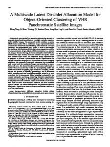
Inference in HLDA - Effects of Hyperparameters Topic Mixing Proportions θd ∼ GEM(m, π) : In the case where θd ∼ GEM (α) the concentration parameter α has the following effect on the Dirichlet Process: • For small values of α the DP concentrates about its base distribution. • For large values of α the DP has greater spread. The depth of the tree (L) is a fixed parameter of the model: The GEM distribution must be truncated after L-1 breaks! This results in an L-dimensional Dirichlet Distribution on topics, where the first L-1 components come from the stick-breaking process, and the last component is the remaining portion of the stick. [7] Two-parameter GEM: In order to have individual control over mean and variance of the GEM distribution let π > 0, m ∈ (0, 1), and Vi ∼ Beta(mπ, (1 − m)π).

I

I

I

I

I

I

0.50-

-

-

-

-

-

0.25-

-

-

-

-

-

0 00 I

I

I

I

I I I ------------

I

I

I

I

I

I

.I .....__ • '---...........______,i____.............., ______,

I

0.10 -

-

-

-

0.05 -

-

-

-

0.00

.

I

II

lJl

I

JI 1

I

.I ,

-I

j-

I I

I

I

I -----------

-

0.04

0.02

o.oo------

0.006------------------------------

0.004

0.002

-4

0

4

-4

0

4

-4

0

4

E[G(A)] = H(A) V[G(A)] =


H(A)(1 − H(A)) α+1 39

Inference in HLDA - Effects of Hyperparameters Model Assumptions on Tree Structure: Even though the model allows for an unbounded branching factor, the values of the hyperparameters will play a role in how the posterior's tree is shaped and distributed. The nCRP's concentration parameter (how likely customers are to sit at the same table across restaurants), γ; and η, the symmetric parameter of the V-dimensional Dirichlet prior on topics control the posterior's preference on the size (branching factor) of the tree. The GEM parameters m and π for the mixing proportions instead control the enforcement of specificity and generality within the tree. [7] • Topic Prior (η) : control over the sparsity of topics on the simplex. Smaller values of η will lead to topics with most of their probability mass on a smaller set of words. If this prior is biased to sparser topics, the posterior will prefer more topics to describe the corpus, thus place larger probability on bigger trees. • nCRP Prior (γ) : If is η small, this implies that the posterior requires more topics to explain the data. A large γ therefore increases the likelihood that documents will traverse new paths when traversing the tree according to the nCRP's specification. • Mixing Proportions (m,π) : The stick-breaking parameters control how many words in each document are likely to come from topics of varying abstraction. o

Large m: the posterior will more likely assign more words from each document to higher levels of abstraction (closer to the root). Can be interpreted as the proportion of general words to specific words in each document, and by extension in the entire corpus.

o Large π: word allocations are less likely to deviate from the setting imposed by the value of m. Therefore it enforces the inferred 'notions' of generality / specificity set by m. A stricter π leads to more 'interpretable' trees. Department of Artificial Intelligence (E3) Jozef Stefan Institute, Ljubjana

40

Inference in HLDA - Effects of Hyperparameters Specificity and Generality: The parameters m and π enforce the notions of specificity and generality to a greater or lesser extent based on their setting. However, irrespective of such a setting there is statistical pressure on the posterior to place more general topics near the root, and more specialized topics near the leaves. [7] •

Each path in the tree includes the root node. By construction of the GEM prior on topic mixing proportions there will be a relatively large probability for documents to select the root node when generating words.

• Therefore, to explain an observed corpus, the topic at the root node will place high probability on words that are useful across all the documents. • Moving down in the tree, recall that each document is assigned to a single path. Thus, the first level below the root induces a coarse partition on the documents, and the topics at that level will place high probability on words that are useful within the corresponding partitions. •

As one descends the tree, the nested partitions of documents become finer. Consequently, the corresponding topics will be more specialized to the particular documents in those paths.


41

Inference in HLDA Hyperparameter Sampling: The values of the hyperparameters are unknown a priori. MetropolisHastings sampling is interleaved with the Gibbs sampler in order to update these values. (This preserves the integrity of the Markov Chain) In particular [7] :

m ∼ Beta(α1 , α2 ) π ∼ Exponential(α3 ) γ ∼ Gamma(α4 , α5 ) η ∼ Exponential(α6 ) Q: Does it make sense to sample hyperparameters? Depends on the goal for which the model is employed. Exploration vs Exploitation. A given setting of the hyperparameters will influence the overall structure of the posterior. This implies that forcing the hyperparameters to assume a given value will 'force' a more predetermined result. It is hence more exploitational : require some metric to determine what constitutes a 'good' tree. Is this context specific? Is this general? On the other hand, letting hyperparameters be sampled aligns itself with an exploratory goal: intrinsic level of specialization/generality and of breath of the tree learned from the data itself. Department of Artificial Intelligence (E3) Jozef Stefan Institute, Ljubjana

42

Inference in HLDA Assessment of Convergence: A useful statistic in determining both the convergence of the Markov chain as well as a local modes of the posterior is the log-likelihood of each sampled state. Conditioned on the hyperparameters, the log probability of all latent variables at any given iteration is computed as [7] :

L(t) = log p

c(1:t)D ,

z(1:t)D ,

w1:D | γ , η, m, π

Local modes of the (empirical distribution) posterior correspond to local maxima of the log-likelihood, therefore the states of the sampler which best describe the posterior are the iterations which correspond to said local maxima. Furthermore, convergence of the chain can be assessed by examining the stationarity of the log-likelihood: the most trustworthy indicators being the Augmented Dickey-Fuller Test as well as the form of the Autocorrelation and Partial Autocorrelation functions. In practice this probability score is computed for a given number of initializations, and the one with the highest score is used as starting point for sampling.


43

Empirical Results

Empirical Results Computational time grows with the number of inferred topics: The entire corpus of 37 million documents cannot be analyzed at once due to the extreme computational and time requirements. Regularity Assumption: Small random samples of the dataset are drawn, and posterior inference is carried out on such corpora. In particular, corpora of 36, 78, and 160 thousand documents are drawn uniformly at random from the original corpus. Although corpora of such sizes are very small compared to the size of the original corpus (0.1% to 0.4%), they are 'large' both in absolute terms as well as relative to each other. By allowing sampling of all hyperparameters for hierarchies of depth 3 and depth 4 on all such samples, the resulting posterior is extremely similar, both in terms of the resulting hierarchy as well as in terms of the values at convergence of the hyperparameters and the functional form of the log likelihood and the likelihood functions for m, π, and η, even though the number of inferred topics is larger for the larger samples, ceteris paribus. This isn't a formal guarantee, however results seem to indicate that for random samples of such magnitude there is enough regularity to be able to both qualitatively and quantitatively compare results.


46

Empirical Results

Size of the random samples: 32K: Number of docs : 32,038 Number of words : 199,556 Total word count : 468,364

150K: Number of docs : 159,815 Number of words : 779,601 Total word count : 2,261,777

76k: Number of docs : 79,916 Number of words : 432,750 Total word count : 1,128,032

300K: Number of docs : 319,660 Number of words : 1,396,182 Total word count : 4,519,612


45

Empirical Results - Format of Results CORPUS: 75K Documents. DEPTH: 4. All hyperparameter sampling enabled. SCORE ITER ETA GEM_MEAN GEM_SCALE SCALING_SHAPE SCALING_SCALE

= 49559717.5402 = 3307 = 6.372e-01 1.461e+00 1.461e+00 1.462e+00 = 0.249407037938 = 3.29535264227 = 0.5 = 0.25

Topic counts summary: 1 Topics at level 0 356 Topics at level 1 485 Topics at level 2 572 Topics at level 3

KEY: [LEVEL OF TOPIC/WORDS IN ALL DOCUMENTS ASSIGNED TO TOPIC/ DOCUMENTS WHICH INCLUDE THIS TOPIC] [0/859303/79916] MANAGEMENT BUSINESS MICROSOFT MEDIA EXCEL,MICROSOFT [1/3147/1222] NOISE 17 JAAR GOED W [2/815/1222] MINING,MINING GAS,INGENIERíA LOGOTIPOS,DISEñO WORD,SUPPLY ERP,ISO [3/222/1222] WORD,ENGLISH,RESEARCH,MARKET 9001,COMARCH TEXTOS,TRADUCCIóN,ESPAñOL,LINGüíSTICA,LENGUAS RECRUITING,TECHNICAL OFFICE,HEALTHCARE,HOSPITALS,INFECTIOUS [1/2747/1198] BIOLOGY,GENE RESEARCH,DOCUMENTARY SANITARIA,INVESTIGACIóN SPECTROSCOPY,PLASMA BANKING,COMMERCIAL [2/741/1198] PRODUCT ENTRY,MARKETING,EVENT EXCEL,POWERPOINT EXPERIENCE,PROJECT DESARROLLO,MANUFACTURA,SAP,ATENCIóN [3/184/1100] MUSIC PRODUCTION,MUSICAL SERVICE,STRATEGIC LAW,CIVIL BREAKDOWN


47

Empirical Results CORPUS: 75K Documents. DEPTH: 4. All hyperparameter sampling enabled.

ADF: -2.925764904568258 p-value: 0.04243287975728056 Critical values: {'1%': -3.433485707610957, '5%': -2.8629252188514385, '10%': -2.5675074259130812} Log Likelihood is Stationary


48


What this means: • For the GEM distribution on topic mixing proportions, goes m from 0.35 to 0.24, whereas π goes from 100 to 3.1. This suggests that while the initial guess of proportion of general words to specific words is correct, the sharp decrease in the value of π suggests that there is a very high tendency to deviate from the imposed setting: some documents may have a large portion of their topic mixture come from the root or depth 1, whereas others may have most of such mass near the leaves. • For the symmetric Dirichlet prior on topic distributions, the root η stabilizes at a value of 0.6, whereas for all other levels below that such a value is 1.46. Such values are relatively small and indicate that the mass of most topics is restricted to less words, the posterior needing more topics to explain the data. Department of Artificial Intelligence (E3) Jozef Stefan Institute, Ljubjana

49



50

Empirical Results 0.03

0.03 0.03

0.06

23.6 3.21 1.56 0.22 0.56 0.28 11.42 3.56 1.5 0. 319 0. 19 0. 16 4.87 0.47 22.44 21.6 20.8 8 20.4 1 7.09 03..4 96 3.0 7 2.8 2.4 1 0.3 7 1 20. 0 19 4 .7 14 . 2 4 6 0 .37 0 .56 0.0.06 19 3 . 61.21.6 26 016 4 4 1 .22.23 00. .94.9 1 012 9 5. 9 13. .7.64 64 111 9 1 11. .3.44. 07

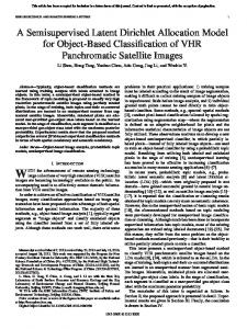
CORPUS: 75K Documents. DEPTH: 4. All hyperparameter sampling enabled.

6

0.0

9 0.0 12

0. 16 0. 16 0. .032 00.1

29.56

22.6 222.44 .6 202.114.1 20.1 20. 19190.74 119 . 1167 .2 11555. . .4.8596 .3 6

1000.0

3 .2 1 15 5.0.983 1144.7585 1144...423 114 .053 1143.7 2 8 133.5 1 .43.2 1 7 1122.6 .39 175 . 12 .9 11 .92 11 7 1.7 1 .67 11 7 11.2 11.02 10.89 10.89 10.43 10 .2 1 10 9..614 1 9.5 8 9.3 .336 99.3 89..7213 8 7 . 5 78.0 8 77..7 8 7.4. 587 67 7 3 66. .8.9.039.4 744

1 2. .97 22. 06 2 .006 2.1.159 2 . 2.2228 .252 22.3 4 22..3 .43374 22.4 7 2.5 2.59 2. 59 2.68 3. 31 3.7 3.751 3.78 3.84

0 00. .1 00.2.11966 00.2.222 00..2.22885 0 . 38 00..4311 .471 00.4 .4 7 00.4 .5 77 00.5 0 .5 0.53 0. 0. 556 6 0. 56 0.6 2 0.6 6 0 .66 0.75 0.78 0.78 0.78 0.78 0.87 0.91 01.90 0. 11.0 . 6 11.0 .0092 11..1 5 11.2 .288 11..2.3444 1 .477 1 .4 3 1 .5 9 11.5621 11. .8.84 1

65 6. .62 9 6 .421 66. .874 5 .7 5 5 5.6 9 5.4 6 55.4 .273 54.0 .87 4.71 4.593 4.4 4 4.3 4.24 4.15 4.12

1. 97 10.4 2 .4 4 2. .06 4 0 0. 9 10.306 2 .781 2 . 18 0 .18 1.8.34 2. 7 2.325 2.3 1 2.3 4 2.4 7 2.4 3 1. 2 7 1.282 0.0 2.5 9 2.5 2 2.68 3.31 3.71 1.22 2.53 3.78 3.84

00. .0 066 97

3.78 0.16 0.16 0.84 2.68

1.

0 1. .44 3 1. 4 9 2. 4 0 0.0 9 0 6 1.7.31 2.1 8 8 0 1..287 0. 8 1.803 7 2.2 5 2.3 1 2.3 4 .12 20.2 5 2.43 2.47 00..2 878 .59 00.6 6 0.09 .75 10.7 5 2.56 2.68 3.31 3.71 0.56 0.6 6 0.06 2.47

5.27 49 31..1 4 .4 0 5 31.6 .22 348 40..2 0.09 4.31 0.25 3.46 0.84

4.12

4.34 4.24 1.28 0.69 0.16 1.47 0.56


16 0. .22 74 0 1.812 11. .2 9 1 .1 8 0 .9 14 .23 14 .5 0 .58 14 .33 140.1239 . 130.84 4 .1 11.81 2 .73 13 .7 101.34 10.0 .37 2 102.3.973 0.0 .42 101.342 0.2 2 0.2 6 0.1

7 12.6 12.39 101.1.568 41 0. 0.03 11.95 11.92 11.77 1 7 10. 6 0.5 0.41 11.27 11.02 10.89 6.31 2.75 1.09 0.34 0.12 0.06 0.03 10.36 9.43 0. 78 10.14 9.61 5.62 3.81 .31 45.0 3 9.33 9.33 6.8 2.3 4 1 8.7 7 4. 3.874 4 8.0 7.7 8 7 7 6 .49 00.0.8.519 06.4 9 00.1.623 00.0.092 7. .069 4 7. 0 06. .1 9 33.5 758 6. .286 74

55 6. 78 2. .47 8 2 .7 9 0 .5 0 9 4 6. 8 6. 1 4 4. 7 1 00.8.31 4 5.7 5 4.6.81 0 9 0.128 11..1652 . 5 0 10..172 2 0.2 4.9

53 1. 81 1. 84 1.

22 0. .83 9 14 0.1 98 . 3 14 4.20.5 1 .58 144.453 1 4.2 4 .09 1 1.181 0 1 2. .73 132.11 1 1.4 8 13.4 4 12.6 2 0.03 0.2 0.16 7 12.6 12.394 11.7 0.44 11.95 11.92 11.77 11.67 11.27 11.02 10.89 6.31 2.75 1.15 0.34 0.12 0.06 0.03 10.36 10.2 10.141 9.6 5.621 3.81 9.3 0.09 9.333 9.33 .84 26.3 8.7 1 7 34.74 8 .84 7 .08 7.5.77 7.4 8 7.4 9 3 7 7. 6. .09 4 6 9 6. .84 3 74

06 0. 55 6. 787 22. .4.789 0 5 . 0 49 6. .21 6 .742 4 .1 1 .74 5 5 40.6.819 0.1.21 3 87 1..41 6 0.5 0 4.9 5.273 5.0 7 4.8 4.629 0.0 1 4.325 0. 3.46 0.84 0.12 4.34 4.24 2.12 2.03 4.12

0.84 0.5 0.53 1.09 3 01.0 .06 9 01.1 .03 8 1.2 5 1.2 4 1. 3 7 01..3035 00..2371 0.8 8 0.2.19.0 01 2 0.1 2 1 1. 9 5 1.

0.03 0.03 0.03 0.03 03 0.03 0. 3 003 0. 0. 0.03 3 3 00.0 .06 .03 00.0 6 0.066 00.0 .0 .06 6 00..0066 0.0 9 0 6 0.0.09 0.0 9 0 .11226 0.0 9 000..1.1166 00. 0 0.

0.78 0.78 0.03 0.75 0.19 0.44 0.16 0.47 0.06 0.84 0.78 1.0 1.0 1.06

0.03

9 0.0

12 16 0. .16 6 0 .1 0

0.

.19 00.3 4 0.56 0.25 0. 31 0.53 0.62 0.66 0.66 0.19 0.03 0.53

23.6 4.99 0.59 0.37 11.42 5.84 4. 0.487 22.447 21.6 21.1 20.4 7 91 4..0 4 3.03 2 .8 2.4 1 200. .317 0 4 1419.7 4.3.26 00. .567 190.0136 1 . 1 7.826 1 6. 9 1 5 15 5.6.92 14 .36 4 .9 8

0.03

0.03 0.03

0.06

6

0.0

9 03

0. 0 0 .1 0. .16 6 16 0. 03 0. 0 16 0 .19 0 .16 0.2.28 0.0 0 8 9 0. .28 3 0. 1 0.0 3 0.422 1 0.4 4 0.4 0.4 7 0.4 7 0.47 0.5 7 0.5 0.53 0.56 0.56 0.53 0.62 0.66 0.66 0.19 0.56 0.78 0.78 0.78 0.62 0.16 0.72 6 0.084 0. 0.94 1.0 .0 1 6 1.0 .91 0.16 01.09 1.099 1.0 5 1.2 8 1.228 1. .34 1 .4 1 .66 0 .81 0 .28 0 .196 1 .1 0 .12 9 1 .5 1 53 5 2 0. 1. .81 4 1 .8 06 1 . 0

0.03

0.03 0.03

6

6 0.006 0.

0.0

0. 1 0.1 9 00.2.03 6 0.2 2 0.2 8 0.3 8 1 0.1 9 0.4 1 0.4 4 0.4 7 0.44 0.47 .12 00.3 7

0.03

0.0

0. 16

51



52

Empirical Results - What can be said about structure? What does this tell us about the given run? (All runs with all hyperparameter sampling enabled exhibit the same behavior). • The posterior seems to prefer a distribution on trees of depth 4 with a relatively large branching factor at the root (many level 1 topics). • At all subsequent levels, there are typically only a few subtopics for each parent topic, implying that if one "lets the data speak" it seems to be the case that there is a lot of diversification at a high level, but then each topic only engenders a few specializations. • Convergence of hyperparameter likelihoods (therefore the log likelihood) as well as hyperparameter values themselves after a burn in period of 2000-2500 iterations seems to suggest that any local mode taken after burn in does reliably explain the underlying structure of the corpus. Issue: The very small value of at convergence implies that specificity and generality aren't well defined. This could mean that some leaf nodes carry more 'importance' than some internal nodes in characterizing the hierarchy. Is this an indication that the corpus is noisy or is there some larger scale implication that indeed specificity and generality cannot be easily defined in the context from which this data comes from? Department of Artificial Intelligence (E3) Jozef Stefan Institute, Ljubjana

53

Empirical Results DEPTH: 3 IT: 5400 SIZE: 36K S: YES

DEPTH: 3 IT: 3000 SIZE: 150K S: YES

DEPTH: 4 IT: 750 SIZE: 36K S: NO



LOG LIKELIHOOD

GAMMA LIKELIHOOD


GEM LIKELIHOOD

ETA LIKELIHOOD 54

Empirical Results DEPTH: 3 IT: 5400 SIZE: 36K S: YES




ETA

GEM

GEM: MEAN: 0.35 -> 0.28 VAR: 100 -> 2.08

GEM: MEAN: 0.35 -> 0.26 VAR: 100 -> 2.3

GEM: MEAN: 0.35 -> 0.27 VAR: 100 -> 3

GEM : MEAN: 0.35 -> 0.24 VAR: 100 -> 3.1

ETA: ROOT: 4 -> 0.63 L 1, 2 : 4 -> 1.5

ETA: ROOT: 4 -> 0.61 L 1, 2: 4 -> 1.5

ETA: ROOT: 4 -> 0.60 L 1, 2, 3: 4 -> 1.5

ETA: ROOT: 4 -> 0.63 L 1, 2, 3: 4 -> 1.5


55

Conclusions and Further Research

This is only half the picture! In the original paper by A. Fedyk, J. Hodson, analysis of firm performance was carried out by using the vector of topic mixing proportions θ, as a covariate. However in order to associate each document int the corpus to the financial entity of provenance, further data than what currently available is required. This part of the research focuses on what can be said about the new 'tool at our disposal': the posterior on the hierarchy, which LDA does not possess by construction. Empirically, for small random samples of the corpus a specific type of tree is preferred by the posterior, along with a set of implications regarding its specificity and generality. The next step: • Assess whether the topic mixing proportions for each document obtained from HLDA yield comparable results to those obtained from LDA with respect to the financial analysis. • Assess whether the levels of the topics and their weights can serve as covariates for the financial analysis. • If either (or both) results of stated assessments are positive, test whether the financial analysis yields different results on random samples of the corpus of significantly different sizes (implicitly tests whether regularity still holds).


57

Hyperparameters and Over/Underfitting Can the hierarchy learned by HLDA be considered a coherent representation of the hierarchy which exists in the context from which the data is obtained? In other words, can the specialization tree learned by the model reflect the underlying structure of specialization of labor in the companies from which the data was obtained? Provided the financial analysis based on the new covariates from HLDA proves feasible, its results may be able to implicitly tell us something about what may constitute a "good" inferred hierarchy. • If such a metric yields positive results with respect to the 'default' inferred hierarchy, then this would indicate the HLDA model is able to accurately capture the structure of the true underlying context of the dataset, and not just of the dataset itself. • If this is not the case however, it may then be worth investigating whether tweaking hyperparameters, thereby forcing the posterior to prefer different hierarchies, yields more consistent results with respect to the second part of the analysis. This would indicate that the learned structure leaving sampling 'as is', is implicitly affected by some phenomenon which cannot be explicitly identified by HLDA. o The depth of the hierarchy, a fixed parameter of the model, should also play a role. Ideally, what can be learned from the second part of the analysis can also be of help in determining this setting.


58

Data from different Time Periods The original dataset has corpora of the type discussed from the 1990's to 2017. If HLDA performed on random samples of corpora from different periods yield similar per-period posterior distributions on trees, and especially similar per-period values at convergence of the hyperparameters, (under the assumption that data collection was performed in a similar manner) this may provide some insight into the evolution of the employment context beyond the datasets themselves. • It is a known fact that in recent years various areas of labor have been 'bleeding' into each other, i.e.: a mathematician relied a lot less on computer science in the 40's, whereas a 'data scientist' wasn't even a profession. • If the topics themselves, or their weights, or the topic mixing proportions all tend to point to a more 'clear cut' posterior for corpora coming from earlier periods this could be interpreted as a manifestation of said 'bleeding in'. • If it is true that for more recent time periods this effect is stronger, this implies that identifying a suitable hierarchy becomes a more difficult task due to greater similarity between documents and other semantic effects such as polysemy.


9

Computational Efficiency vs Integrity It is experimentally proven that Gibbs sampling, and MCMC methods in general, do not tend to scale well when approximating posteriors which arise from hierarchical nonparametric models. • More recently, variational inference has shown to be an alternative which generalizes better to datasets of bigger sizes. • The algorithm is single-core: adapting it to use multiple threads or even the GPU may help in reducing the average time it takes for posterior inference. • Computational time and memory usage increases with the number of topics (implicitly with the size of the dataset as more topics are typically learned with more data). The main drawback is the typically very large dimensionality of the topic distributions (vectors of length 100,000 to 1 million depending on the corpus). •

Without attempting to modify the algorithm itself, one could attempt to apply some kind of dimensionality reduction approach such as porter stemming. The issue would then be one of: does sacrificing the integrity of my dataset for more efficient computation interfere with how specificity and generality are handled by HLDA?


60

References

[1]

H. Kamper, "Gibbs sampling for fitting finite and infinite Gaussian Mixture Models," 2013.

[2]

P. Resnik and E. Hardisty, "Gibbs Sampling for the Uninitiated," College Park, 2010.

[3]

Y. Whye Teh, M. I. Jordan, M. J. Beal and D. M. Blei, "Hierarchical Dirichlet Process," 2005.

[4]

X. Yu, "Hierarchical Dirichlet Process: A Gentle Introduction," College Park, 2009.

[5]

Y. Haiyan, "Hierarchical Topic Models".

[6]

J. I. Michael, "Dirichlet Processes, Chinese Restaurant Processes and All That," Berkeley, 2005.

[7]

D. M. Blei, T. L. Griffiths and M. I. Jordan, "The Nested Chinese Restaurant Process and

Bayesian Nonparametric Inference of Topic Hierarchies," Journal of the ACM, pp. Vol 57, No. 2, Article 7, 2010. [8]

J. Paisley, C. Wang, D. M. Blei and I. M. Jordan, "Nested Hierarchical Dirichlet Process," Journal

of Pattern Analysis and Machine Intelligence, pp. Vol. X, No. X, XXXX. [9]

J. Steinhardt and Z. Ghahramani, "Flexible Martingal Priors for Deep Hierarchies".

[10] C. Wang and D. M. Blei, "Variational Inference for the Nested Chinese Restaurant Process," Princeton.


62

[11]

E. P. Xing, Z. Sheikh and A. Beutel, "Bayesian Nonparametrics: Hierarchical Dirichlet

Process," 2013. [12] Y. Whye Teh, "Bayesian Nonparametrics," Tubingen, 2013. [13] Y. Whye Teh, "A Tutorial on Dirichlet Processes and Hierarchical Dirichlet Processes," London, 2007. [14] D. M. Blei, M. I. Jordan, T. L. Griffiths and J. B. Tenenbaum, "Hierarchical Topic Models and the Nested Chinese Restaurant Process," 2003. [15] J. Hodson and A. Fedyk, "Trading on Talent: Human Capital and Firm Performance," Jozef Stefan Institute, Ljubljana, 2017. [16] M. I. Jordan, A. Y. Ng and D. M. Blei, "Latent Dirichlet Allocation," Journal of Machine Learning Research 3, pp. 993-1022, 2003. [17] Y. W. Teh, "Bayesian Nonparametrics," Tubingen, 2013. [18] Y. W. Teh, "Dirichlet Process," Oxford University, 2010. [19] Y. W. Teh, M. I. Jordan, M. J. Beal and D. M. Blei, "Hierarchical Dirichlet Process," 2005. [20] F. S. Thomas, "A Bayesian Analysis of Some Nonparametric Problems," The Annals of Statistics, pp. 209-230, 1973. [21] B. Fang, "Introduction to the Dirichlet Process,", 2016. Department of Artificial Intelligence (E3) Jozef Stefan Institute, Ljubjana

63