High bandwidth, Low Latency Global Interconnect Christer Svensson* and Peter Caputa Dept. of Electrical Engineering, Linköping University, 581 83 Linköping, Sweden. ABSTRACT Global interconnects have been identified as a serious limitation to chip scaling, due to their limited bandwidth and large delay. A critical analysis of intrinsic limitations of electrical interconnect indicates that these limitations can be overcome. This basic analysis is presented, together with design constraints. We demonstrate a scheme for this, based on the utilization of upper-level metals as transmission lines. A global communication architecture based on a global mesochronous, local synchronous approach allows very high data-rate per wire and therefore very high bandwidth in buses of limited width. As an example, we demonstrate a global, 250µm wide bus with a capacity of 160Gb/s in a nearly standard 0.18µm process. Keywords: Interconnect, low latency, high bandwidth, global
1. INTRODUCTION Integrated circuit interconnect has been considered a showstopper for process scaling because of their RC delays1-5. However, it was early noticed that the RC-delay could be considerably reduced by utilizing upper level, thicker metals for long interconnects3. It was in fact predicted that global synchronism could be maintained until the feature size reached 0.3µm. Today, we know that high speed interconnects must be described by models which include not only R and C but also inductance and skin effect4-6. The first thought is that this will make the situation worse, but we found that it is not so. In this paper we will show that well designed, highly lossy, long interconnects may show reasonable delays of the order of twice the delay compared to the velocity of light delay, and allow high data rates. Contemporary VLSI developments can be characterized as System on Chips (SoC). A SoC is often designed as a number of predefined blocks, or IP-cores, for example processors, DSP’s or memories, which are integrated into one chip. A key issue in SoC design is how to facilitate an effective communication between the various IP-cores. Traditionally, this communication constitutes custom buses and glue logic, often demanding large design and verification effort. A new trend is to utilize Networks on Chip (NoC)7-10, both in order to mitigate the design and verification effort and to increase the available communication bandwidth between the IP-cores. In the present paper we will use the NoC model for SoC communication to demonstrate an efficient utilization of upper level metal interconnect.
2. BASICS OF WIRES The performance of wires or bundles of wires (buses) can be described in terms of four parameters, delay (or latency), maximum data-rate, crosstalk and power consumption. We will first discuss wire modeling in general and then return to these four parameters. The most general wire model is the transmission line model (The telegraph equation)4. This model is only valid for wires with a well defined return path, as for example twisted pairs, coaxial cables, striplines or coplanar waveguide, see fig. 1. As we are interested in high-performance wires, we will only consider such well-defined lines in the following, mainly microstrip. The wire is thus described by its transfer function, H, and characteristic impedance, Zc (complex), calculated from inductance, l, capacitance, c, and resistance, r, per unit length, wire length, L, and including skin effect6,11. H is the transfer function of a wave moving through the wire, and is given by:
H = e− *
( jωl + r ) jωc L
[email protected], www.ek.isy.liu.se
(1)
Ground planes
Microstrip
Coplanar waveguide
Fig. 1. Microstrip and coplanar waveguides.
Zc is the relation between voltage and current in each wave on the wire (one wave in each direction):
Zc =
jωl + r c
For high frequencies Zc approaches l included in r. r can then be expressed as:
(2)
c , which we will term Z0. Also at high frequencies, skin effect should be
r = rDC + rs (1 + j ) ω
(3)
where the second term describes skin effect (the j-term describes the inductive part of the skin effect). Also dielectric loss may be included in these formulas, through a complex and frequency dependent dielectric constant in c11, but dielectric loss is not considered important inside chips. If the wire is connected to a driver with output impedance ZS and loaded by an impedance ZL, we may express the total transfer function from driver emf to voltage over the load as G:
G (ω ) =
2Z L H § § · · Z Z Z L ¨¨1 + H 2 + s (1 − H 2 )¸¸ + Z c ¨¨1 − H 2 + s (1 + H 2 )¸¸ Zc Zc © © ¹ ¹
(4)
Eq. (4) is obtained from circuit equations, combined with the two waves on the transmission line4. We may note, that for perfect terminations, ZL=ZS=ZC, G=H/2. Further, for ZS=ZC and ZL=∞, G=H, that is we get the full amplitude from the source appearing at the far end of the wire. In order to better understand the wire behavior in various circumstances, it is useful to analyze the step response of its transfer function, h, which can be found from the inverse Fourier transform of H11. In fig. 2 we show h for the case of 50% wire attenuation. We note that the step response is characterized by an initial delay, which corresponds to the velocity of light delay, a step with limited height, which height corresponds to the wire attenuation, and finally a slow rising path approaching 1, which corresponds to RC charging of the wire. Taking skin effect into account will make the step slower (the frequency-dependence of the skin-effect gives rise to signal distortion). For most integrated circuit wires, the attenuation is very large, making the RC-charging (RC-behavior) dominate the behavior, and they have an open far end, making ZL purely capacitive (CL). For this case Eq. (4) is reduced to the Elmore delay expression12, describing the wire with a π-circuit, consisting of a series resistor with the wire DC-resistance and two capacitors, half the wire capacitance each:
1 0.9
Normalized amplitude
0.8 0.7 0.6 0.5 0.4 0.3 0.2 0.1 0 0
0.5
1
1.5
2
2.5
3
3.5
Time, seconds
4 −9
x 10
Fig. 2. Step response of a wire transfer function, solid: without skin effect, dashed: with skin effect (The weak ringing is a mathematical artifact).
§ §C ·· t Elmore = ¨¨ RS (C S + C w + C L ) + Rw ¨ w + C L ¸ ¸¸ ln 2 © 2 ¹¹ ©
(5)
where RS and CS is the source resistance and capacitance and Rw and Cw is the wire resistance and capacitance respectively. This is then the traditional view of integrated circuit wires, characterized with large delays (much larger than delays related to the velocity of light). For the opposite case, wires with relatively small attenuation, the step in fig. 2 dominates (LC behavior), and the wire delay can be considered to be:
td =
L vd
(6)
where vd is the velocity of light in the actual dielectric used, vd=v0/n, where v0 is the velocity of light in vacuum and n is the refractive index, given by n = ε r , εr being the relative dielectric constant. Low loss wires thus have the smallest possible delay allowed by physics. The borderline between the two cases, RC-behavior and LC-behavior occur for an attenuation of 50% (considering that we measure delay from the step launch time to the time at which the signal reaches 50% of its final value at the far end). Using the “classical” loss formula4:
H ≈e
−
rL 2Z 0
(7)
gives the constraint for the wire to behave as a transmission line:
rL ≤ 2 ln 2 Z0
(8)
Returning to the full expression for G, eq. (4), we may calculate its step response, g, in the same way as we calculated h. This was done for ZS=Z0, ZL=∞ and 50% loss, and shown in fig. 3. We note that g(t) (or the step response S(t)) is in fact much steeper than h(t). Particularly, h(t) show a very long tail which is very detrimental for the data-rate, as it gives rise
1
S(t)
Normalized amplitude
tB 0.8
ifft(H) 0.6
td 0.4
0.2
0 1
1.5
2
2.5
−9 Time, seconds x 10 Fig. 3. Theoretical step response, S(t), of an open wire driven by a terminated driver, G, compared to the step response of the wire transfer function, H.
to intersymbol interference (ISI). ISI means that one symbol affects subsequent symbols through the long tail. The fact that g(t) is much better in this respect is caused by the difference between the actual characteristic impedance of the wire, ZC and its high frequency value, Z0, causing an enhancement of the input voltage at the input edge. This is an important effect, which we utilize in this work. Let us now return to the four performance parameters of the wire. The delay, or latency, of the wire is thus given either by the velocity of light of the actual dielectric used or by the RC delay. Velocity-of-light delay, eq. (6), is valid for wires with loss less than about 50%, i.e. for wires fulfilling the constraint eq. (8) above. On the borderline, we need to add part of the wire risetime to the delay, making it about double L/vd. For these wires, repeaters do not improve delay, as delay cannot be less then velocity-of-light delay anyway. For wires with larger resistance, the delay is given by the RC-delay formulas, eq. (5), often considerably larger then the velocity-of-light delay. We will only consider wires with velocity-of-light delay in the following. The maximum data-rate of a wire is controlled by its step response, S(t). In a lossy wire the data-rate is limited by the intersymbol interference (ISI) imposed by the transfer function of the wire. The effect of ISI can be quantified as the minimum eye-opening of the eye-diagram of the received signal. This minimum eye-opening (the smallest difference between a “0” and a “1”) occurs for a single zero and a single one, and is given by 2S(T)-1, where S(T) is the step response of the transfer function and T=1/B is the data period of a binary data stream with bit-rate B6. For a lossless transmission line B is infinite, but with loss the value is lower. It turns out that the step response of an open wire, driven by a driver with output impedance Z0 or less, is better than the step response of the transfer function itself, as discussed above in connection to fig. 3. As we are interested in the time at which S(t) is relatively large (typical 0.8, tB in fig. 3), the two curves in fig. 3 yields very different data-rates. We may interpret the upper curve as a result of pre-emphasis, i.e. the input voltage to the wire is enhanced in the beginning of the bit13 (in this case occurring as a result of a fixed driver impedance compared to a frequency-dependent characteristic impedance of the wire). This effect can be further emphasized by choosing a lower driver impedance, see the example below. If we consider a bundle of wires, we also need to consider crosstalk. For a simple bundle of parallel wires, the worst case crosstalk occurs when the two neighboring wires have data edges opposite to the edge on the actual wire. The amount of crosstalk is controlled by the mutual inductances and capacitances between the neighbors, but also with transmitter and receiver impedances4. The amount of crosstalk can be controlled by controlling the spacing between neighboring wires, or by using each second wire in the bundle as a grounded shield14. We have only determined crosstalk by simulations, see the example below.
Power consumption of the wire, finally, is proportional to voltage swing, Vs (here assumed equal to the supply voltage) squared. For a terminated transmission line (far end terminated by Z0), the input impedance is always Z0, making its power consumption independent of wire length (assuming random data):
Vs2 P= 2Z 0
(9)
For an open wire, the power consumption is lower and given by6:
P=
Vs2 8Z 0
for td>T/2
(10)
P=
Vs2 t d 1 = BC wVs2 4Z 0 T 4
for td