May 19, 1993 - Appendix A: Solving Equations for High Dimensional Objects 62 ..... Ratios of these volumes become significant for estimating statistical likeli-.
High-Dimensional Linear Data Interpolation Russell Pflughaupt May 19, 1993 MS report under direction of Prof. Carlo H. Séquin
Abstract This report explores methods for interpolating across highdimensional data sets. We describe and evaluate algorithms designed for problems with 100 to 10,000 points in dimensions 2 through 40. Specialized algorithms that attempt to take advantage of properties of locality are shown to be less efficient than generalized algorithm such as gift-wrapping and linear programming. In addition, this report contains an accumulation of information on the properties of high-dimensional spaces.
Table of Contents 1 Introduction
1
2 Why the Problem is Difficult
3
The D Dimensional Simplex 3 “Typical” Number of Simplices Attached to a Vertex in D Dimensions 4 "Typical" Number of Nearest Neighbors in D Dimensions 5 Maximum Number of Simplices in D Dimensions with N Vertices 5 Volumes of High Dimensional Objects 7 Conclusions 14
3 Finding the Enclosing Delaunay Simplex 3.1 A Backtracking Simplex Finder 3.2 A Non-Backtracking Simplex Finder 3.3 A Local Delaunay Simplex Finder 3.4 A Global Delaunay Simplex Finder
15 17 20 31 44
4 Extrapolations
52
5 Outstanding Issues
58
6 An Alternative Approximation Technique
60
7 Conclusion
61
Appendix A: Solving Equations for High Dimensional Objects 62 Appendix B: Kd-Trees in High Dimensions
65
Bibliography
68
1 Introduction There are situations where one would like to have a real-time simulation model of a complicated system such as a high-performance airplane or rocket engine for ‘what-if' type experiments before actual changes are induced in the operational state of the engine. A few thousand test points describing the state of the engine in a high-dimensional data space corresponding to the various variables measured (gas mixture, speed, pressure, temperature at various points) may have been gathered by actual measurements or by lengthy in-depth systems simulations on a highpowered computer. For actual use, one would like to interpolate (and perhaps extrapolate) the given data points in a robust manner. Although interpolation of data sets is a well known problem that has largely been explored in great detail, an area that has not been sufficiently explored is how dimensionality affects this problem. A conceptually straightforward approach to interpolation in 2D is to simply triangulate the data and use the values at a triangle’s vertices to interpolate over its interior. However, a triangulation scheme must be found that is both consistent and “well-behaved”. Consistency is required so that a given data location is always interpolated in the same triangle with the same vertices. Being “well-behaved” means that every vertex of a triangle is in some sense “near” to every point enclosed by that triangle. It is easy to imagine an inconsistent triangulation which depends on the order in which the data points were originally presented. Likewise, it is easy to imagine a poorly behaved triangulation which produces long, skinny triangles. This would result in interpolations that use far away data points rather than closer ones. Two methods of triangulation are possible: In the first, some reasonably good global triangulation would be computed, written to disk, and provided with an efficient index for access. In the second, the data set would be kept in memory and a canonical triangulation is computed on demand in the neighborhood of each query point. Given an efficient indexing scheme, access to a fixed triangulation on disk may have response times measured in milliseconds. However, constructing the complete global triangulation may take weeks. This paper investigates local, on-the-fly triangulations. One would hope that an on-the-fly triangulation could be found that was both efficient in running time and storage requirements. This method has no initial cost for computing the global triangulation, but the response time might be much slower than that of the precalculated triangulation. Keeping a cache of most recently used triangles is one method to speed up nearby queries. In choosing a local triangulation scheme, particular care must be taken to guarantee consistency. The obvious choice is the Delaunay triangulation. Ignoring the special case of co-circular points, the Delaunay triangulation will always produce a canonical triangulation that is based solely on the data points. The Delaunay triangulation can be defined as “the unique triangulation such that the circumcircle of each triangle does not contain any other point in its interior.” [PREP85]
1
Figure 1: Example of Delaunay triangulation (left) and non-Delaunay (right) This implies a very desirable property. Given a Delaunay triangle on a set of points, new points can be added and the triangle will remain Delaunay so long as no new point falls within its circumcircle. Stated another way, a triangle can be verified to be a Delaunay if its circumcircle contains no points other than its own vertices. This property allows local triangulations to be created that can be guaranteed to be Delaunay by checking for the absence of any other points within each circumcircle. Up until now, we have limited ourselves to a language that can only describe objects in two dimensions. A more general language needs to be adopted that can refer to higher dimensional objects. We could let triangles become simplices, triangulations become hyper-tessellations, lines become hyperplanes, circles become hyperspheres, etc. However, much of this tends to obscure the underlying concepts. Unless explicitly stated otherwise, throughout the rest of this report we will assume simplices, triangulations, planes and spheres to all refer to their D-dimensional counterparts. Notice that the definition of a Delaunay triangulation remains essentially unchanged: the unique triangulation such that the circumsphere of each simplex does not contain any other point in its interior. In dimension D, a simplex is uniquely determined by its D+1 vertices. Likewise, a sphere in dimension D is uniquely determined by D+1 points that lie on its surface. This extension allows the Delaunay triangulation to be used in problems of arbitrary dimension.
2
2 Why the Problem is Difficult1 The purpose of this chapter is to expose the reader to aspects of high dimensional geometry. Much of what is presented in this chapter was developed and/or researched after our algorithms for finding a Delaunay simplex enclosing a query point had been completed. It is presented now to provide the reader with a context from which she may better understand the failings of the algorithms in the next chapter. It is also hoped that this information will prove useful to researchers in related problem areas. We start by examining the D-dimensional simplex and calculate the number of nearest neighbors a vertex has, how many simplices are attached to each vertex, the total number of expected simplices in D dimensions with N data points, and the volumes of high dimensional objects.
The D Dimensional Simplex Certainly a good place to start in the tour of high dimensionality is with an examination of the D dimensional simplex. A simplex can be thought of as a D dimensional “triangle”. In 0D this would be a point, in 1D an edge, in 2D a triangle, in 3D a tetrahedron or cell, etc. A simplex in D dimensions requires D+1 vertices. Anything less would produce a simplex of less than D dimensions (i.e. 3 vertices in 3D just produces a triangle oriented in 3-space).
0D
1D
2D
3D
4D
Figure 2: Simplices in D dimensions The number of 1D edges for a D dimensional simplex is D
∑i
( D+1 ) D 2
or
i=1
This formula can readily be derived from the recursion that if a D+1’st vertex is added to a D-1 dimensional simplex, new 1D edges will be added to the new vertex from all the original D vertices (adding D more 1D edges). A similar recursion gives the number of 2D faces. If a D+1’st vertex is added to a D-1 dimensional simplex, new 2D faces will be added to the new vertex from the original edges (add1. This Chapter might more aptly be called The Curse of Dimensionality [EUBA88].
3
ing D(D-1)/2 more 2D faces). In general, the number of 2D faces in a D dimensional simplex is the number of 1D edges in a D-1 dimensional simplex plus the number of 2D faces in a D-1 dimensional simplex. This is ( D+1 ) D ( D-1 ) 6 3D cells are like everything else. Each time a vertex is added, the number of 3D cells increases by the number of 2D faces on the original simplex. In general, the number of 3D cells in a D dimensional simplex is the number of 2D faces in a D-1 dimensional simplex plus the number of 3D cells in a D-1 dimensional simplex. This is ( D+1 ) D ( D-1 ) ( D-2 ) 24 A pattern begins to emerge. Every D dimensional simplex is made up of lower dimensional simplices. Let S represent the dimension of the simplices you wish to count on a D dimensional simplex. Remembering that vertices are 0 dimensional simplices, the number of S dimensional simplices on a D dimensional simplex is ( D+1 ) ! 1 ⋅ S+1! ( D-S ) !
or
D+1 S+1
“Typical” Number of Simplices Attached to a Vertex in D Dimensions An interesting aspect of dimensionality is the number of simplices a “typical” vertex in a data set would be attached to. Given an actual set of vertices, this can be computed exactly using a Vornoi diagram. However, we are more interested in general guidelines for high dimensions. Therefore we’ll derive the typical number using an infinitely large regular tessellation, since the average number must be exactly the same as if the tessellation were irregular. We’ll start by taking a 3 dimensional cube and triangulating its 6 surface faces into 12 triangles. If you were to take a point inside the cube and construct simplices using this point and the triangles on the surface of the cube, there would be 12 simplices. However, moving this point to one of the cube’s corners forces the 6 simplices adjacent to this corner to collapse. This leaves half of the triangulated cube faces as “bottom” faces for simplices with their tops at that corner. With 2 simplices per face on the cube, there are 3*2 simplices. We can now recurse using this 3 dimensional cube. The 4 dimensional cube has 8 boundary cubes. Break half of these into the previously defined 6 3D simplices which then act as the bottoms for 24 4D simplices (with a shared vertex at one corner). The 5 dimensional cube has 10 boundary hypercubes resulting in 5*24=120 5D simplices. In general, the number of simplices in a cube is D!. Since each simplex is attached to D+1 vertices and since each cube accounts for 1 vertex in the grid, the typical number of sim-
4
plices attached to a vertex in D dimensions is (D+1)D!
or
(D+1)!
“Typical” Number of Nearest Neighbors in D Dimensions To calculate the typical number of nearest neighbors in D dimensions we’ll use the same tessellation described in the previous section, “Typical” Number of Simplices Attached to a Vertex in D Dimensions. We count the number of edges in a single cube and weigh them by the amount of sharing they experience with adjoining cubes. For example, a 3D cube has 12 boundary edges that are shared with 3 other cubes each, 6 edges embedded in the 6 faces of the cube that are shared with 1 other cube each, and 1 internal edge which is shared with no other cubes. Since there are 2 vertices for every edge, the typical number of nearest neighbors in 3 dimensions is 2× (
12 6 + + 1 ) = 14 4 2
In general, the edges of a D dimensional cube get shared 2 D-1 fold and the edges embedD ded in every face of dimension J get shared 2 D-J fold. Since a D dimensional cube has 2 D-J ( ) J features of dimension J, we need only sum from J=1 to J=D and multiply by 2. 2×
D D D D ( ) + ( ) +... + ( ) + ( ) 1 2 D-1 D
= 2 D+1 − 2
This number is considerably larger than the equivalent number for densest sphere packing because we are not constrained to have all nearest neighbors to be equidistant from each other1.
Maximum Number of Simplices in D Dimensions with N Vertices Paschinger [PASC82] and Seidel [SEID82], [SEID87] independently proved that the upper bounds for the number of i-dimensional faces µ i in a D dimensional Vornoi diagram with N vertices is:
µ i ( N, D ) =
C D − i ( N, D + 1 ) − 1 C D − i ( N, D + 1 )
i=0 01, the additional points are used to force the next gift-wrapping plane to be coplanar with a set of edges from the partially built up simplex. Nevertheless, we are left with D+1-k degrees of freedom to choose. A heuristic is used to direct the gift-wrapping to swing towards the query point. We start by constructing the vector from the center of mass of the partially built up simplex to the query point. This vector is called best_vec because it represents the direction with the highest likelihood of forming a Delaunay simplex enclosing Q. Specifically, we use one degree of freedom to turn the normal vector of the current gift-wrapping plane towards best_vec (i.e. make sure that the sign of the dot product of the two vectors be positive). The remaining D-k constraints are formed using the relative magnitudes of the components of best_vec. If component i of best_vec has the largest absolute value and com-
33
ponent j has the second largest absolute value, then we constrain ni =
best_vec i ⋅n best_vec j j
For example, if best_vec=[9, -2, 5, -13, -3] and D-k=3, we constrain n 4 = −
13 9 ⋅ n 1, n 1 = ⋅ n 3, 9 5
5 and n 3 = − ⋅ n 5 . 3 Main Loop: Given a convex hull facet of D+1 points, project these points down to D dimensional space and use BarycentricCoords() to see if Q lies inside the Delaunay simplex defined by them. If Q is inside (by testing for all coordinates in [0, 1]) then we are done, otherwise we need to giftwrap on the D+1 dimensional paraboloid about the sub-facet for which Q has the most negative barycentric coordinates (the corresponding antipodal point of the facet will be discarded). Go back to the Main Loop. There is one problem in using the convex hull to solve for Delaunay simplices. Gift-wrapping solves for the entire convex hull of the paraboloid. The gift-wrapping plane can swing over the top of the paraboloid yielding simplices that are not Delaunay. This can only occur when an attempt is made to gift-wrap about a sub-facet of the D-dimensional convex hull of the points in point_list (i.e. the upper rim of the partial paraboloid). We require a method to detect when this has occurred, so that either more points can be fetched into point_list or a determination can be made that Q is outside the global convex hull. Fortunately, this test is fairly trivial. If a gift-wrapping plane partitions space such that the point (0, 0, ..., 0, + ∞ ) is not on the same side as all the data points, then the plane has wrapped over the top of the paraboloid. This test is simply to check that the signs returned by TestPointVsPlane() for (0, 0, ..., 0, + ∞ ) and for the center of mass of the paraboloid are the same. D+1
facet of D+1 dimensional convex hull which does not correspond to a Delaunay simplex
Q Figure 12: Example of Convex Hull facet which is not a Delaunay simplex
34
Analysis: We initially had high hopes for this algorithm. The first two algorithms operated on general simplices. This algorithm operates on only Delaunay simplices. Surely the number of Delaunay simplices in the entire data set must be much less than the number of general simplices in the entire data set. This should greatly reduce the number of “walks” (or “wraps”) required to eventually enclose the query point. Unfortunately, as dimensionality increases, guaranteeing that a simplex is Delaunay requires looking at higher and higher percentages of the data set. As was mentioned in Section 2.2, the ratio of the volume of a sphere relative to the volume of an enclosed simplex is superexponential. The circumsphere from each Delaunay simplex encloses more and more volume in higher dimensions. We are required to fetch a higher percentage of points from the data set, so that those points that could possibly lie within a simplex’s circumsphere are contained in point_list. Statistics were gathered by running this algorithm over 100 randomly chosen query points. It was shown in Section 3.2 that as dimensionality increases, it is less and less likely for a query point derived from the same random distribution as the data set to actually lie inside the convex hull of the data set. For this algorithm, the query point was derived using the data set in the following manner: chose a single random point from the data set and use GetClosest() to fetch the D+2 nearest neighbors to this point (note that this effectively returns the D+1 closest points and the point itself). The center of mass of these D+2 points will be used as a query point1. This construction guarantees that each query point will lie within the convex hull of the data set and it also produces query points that will tend to have a distribution similar to that of the data set. Below are statistics measuring the average number of points that need to be fetched to guarantee that by the time an enclosing Delaunay simplex is found, every simplex in the “walk” towards Q was a Delaunay simplex. These statistics were gathered by keeping track of the largest r1+r2 (see Figure 9) encountered in the Delaunay “walk” towards each Q (with point_list containing all of the data points). It is then straight forward to count the number of data points within r1+r2 from Q. The first two tables show the average number of points needed to guarantee that every gift wrap produced Delaunay simplices. The next two tables and graph show this same data, except expressed as a percentage of the size of the entire data set.
1. The choice of using D+2 points is admittedly ad hoc. Using less than D+1 points would not allow the data space to be sufficiently explored. Using more than D+2 points would cause the constructed query point to migrate towards the center of mass of the data set.
35
Table 15: Average Number of Points Needed to Guarantee Delaunay (Uniform) Dim
128
256
512
1024
2048
4096
8192
2
4.0
3.8
4.8
3.8
4.3
4.0
3.6
5
15.8
26.6
15.6
20.9
25.8
65.0
23.1
10
38.4
52.9
65.8
67.6
82.7
92.2
183.2
20
78.5
94.8
119.6
133.2
206.7
224.6
295.5
40
123.7
214.2
313.3
392.0
503.4
513.7
592.7
Table 16: Average Number of Points Needed to Guarantee Delaunay (Gaussian) Dim
128
256
512
1024
2048
4096
8192
2
3.8
4.6
4.2
4.0
3.8
3.9
3.6
5
18.9
23.5
23.2
21.9
22.8
21.0
17.5
10
44.4
53.9
68.7
83.6
74.8
74.5
111.3
20
93.4
154.5
170.5
206.2
247.6
275.1
196.9
40
126.6
235.3
327.5
509.4
663.0
879.2
760.0
Table 17: Average Percent of Data Set Needed to Guarantee Delaunay (Uniform) Dim
128
256
512
1024
2048
4096
8192
2
3.11
1.49
0.94
0.37
0.21
0.09
0.04
5
12.31
10.38
3.05
2.04
1.26
1.59
0.28
10
29.98
20.67
12.85
6.60
4.04
2.25
2.24
20
61.34
37.01
23.36
13.00
10.09
5.48
3.61
40
96.62
83.68
61.20
38.28
24.58
12.54
7.23
36
Table 18: Average Percent of Data Set Needed to Guarantee Delaunay (Gaussian) Dim
128
256
512
1024
2048
4096
8192
2
2.99
1.78
0.82
0.39
0.19
0.09
0.04
5
14.76
9.19
4.53
2.13
1.11
0.51
0.21
10
34.65
21.07
13.43
8.16
3.65
1.82
1.36
20
72.96
60.37
33.29
20.13
12.09
6.72
2.40
40
98.87
91.92
63.96
49.74
32.37
21.46
9.28
Average Percent to Guarantee Delaunay (Uniform)
Average Percent to Guarantee Delaunay (Gaussian)
100
100
40
40 80
80
20
GRAPH 8
60
60
20 40
40
10
10 5 2
20 0 128
20
5 2
0 256
512
1024
2048
4096
8192
128
256
512
Number of Data Points
1024
2048
4096
8192
Number of Data Points
The following two tables show the maximum observed number of points needed to guarantee that every gift wrap produced Delaunay simplices for our 100 random query points. The next two tables and graph show this same data, except expressed as a percentage of the size of the entire data set. Table 19: Maximum Observed Number of Points Needed to Guarantee Delaunay (Uniform) Dim
128
256
512
1024
2048
4096
8192
2
14
17
36
12
22
13
17
5
74
115
129
222
677
4087
309
10
115
250
424
405
913
1199
3705
20
128
255
473
762
2034
2581
5864
40
128
256
500
1024
2046
2696
5627
37
Table 20: Maximum Observed Number of Points Needed to Guarantee Delaunay (Gaussian) Dim
128
256
512
1024
2048
4096
8192
2
10
30
28
15
13
14
10
5
113
141
250
249
254
135
97
10
116
226
304
857
423
528
983
20
128
254
369
716
1228
1243
1103
40
128
256
510
968
1899
3711
3240
Table 21: Maximum Observed Percent of Points Needed to Guarantee Delaunay (Uniform) Dim
128
256
512
1024
2048
4096
8192
2
10.94
6.64
7.03
1.17
1.07
0.32
0.21
5
57.81
44.92
25.20
21.68
33.06
99.78
3.77
10
89.84
97.66
82.81
39.55
44.58
29.27
45.23
20
100.00
99.61
92.38
74.41
99.32
63.01
71.58
40
100.00
100.00
97.66
100.00
99.90
65.82
68.69
Table 22: Maximum Observed Percent of Points Needed to Guarantee Delaunay (Gaussian) Dim
128
256
512
1024
2048
4096
8192
2
7.81
11.72
5.47
1.46
0.63
0.34
0.12
5
88.28
55.08
48.83
24.32
12.40
3.30
1.18
10
90.62
88.28
59.38
83.69
20.65
12.89
12.00
20
100.00
99.22
72.07
69.92
59.96
30.35
13.46
40
100.00
100.00
99.61
94.53
92.72
90.60
39.55
38
Maximum Percent to Guarantee Delaunay (Uniform)
80
40 20
60
10
100
Maximum Percent to Guarantee Delaunay (Gaussian) 100 80
40
GRAPH 9
60
10 40
20
40
5
20
2
0 128
256
512
5
20
2
0 1024
2048
4096
8192
128
Number of Data Points
256
512
1024
2048
4096
8192
Number of Data Points
We are forced to the conclusion that the “local” nature of a Delaunay triangulation does not lend itself to exploitation in higher dimensions. Global information must be used at every step to guarantee the Delaunay status of simplices. This is why we have waited so long in describing a method for choosing M. It is evident that in high dimensions M must be equal to the number of points in the entire data set (except for extremely large data sets). Even though the first two algorithms worked with general simplices, there still is the conversion process to Delaunay (which we never developed) which must use global information. The current algorithm can be easily modified so that the paraboloid is computed just once at the center of mass of the data set. Instead of fetching M nearest neighbors to Q, just find the closest point P to Q. Use P as the initial point to gift-wrap about to find an initial convex hull facet. However, instead of starting with a plane perpendicular to the D+1’st dimension, use a plane tangent to the paraboloid at P (how to construct this plane is discussed in detail in the next section). The remainder of statistics in this section were gathered by fetching all the data points into point_list for every query point (setting M=N) rather than changing the algorithm as described in the preceding paragraph. The results will be exactly the same except for a slight discrepancy in the execution time. Because we fetched the data points outside the timing loop, there is no cost for finding the closest point P to Q (it’s just at the head of point_list). The changes described in the preceding paragraph require finding the closest point P to Q. Using a brute force linear search through the data set would take O(N·D) work. This is the same as one gift-wrap step. The following two tables and graphs show the average number of gift wraps used as a function of dimensionality and number of data points. Note that the minimum possible number of gift wraps is equal to D (this many is required to find and initial convex hull facet). Every gift wrap above D finds a new Delaunay simplex closer and closer to a query point. Each gift wrap requires O(N·D) work.
39
Table 23: Number of Gift Wraps (Uniform) Dim
128
256
512
1024
2048
4096
8192
2
2.1
2.1
2.1
2.1
2.2
2.1
2.1
5
7.0
7.7
7.3
6.8
7.3
6.9
7.0
10
16.8
18.2
18.7
20.2
20.1
20.9
22.1
20
35.6
39.6
44.6
48.1
55.9
58.9
63.2
40
75.2
89.3
101.9
113.0
128.7
140.0
149.9
Table 24: Number of Gift Wraps (Gaussian) Dim
128
256
512
1024
2048
4096
8192
2
2.1
2.1
2.1
2.2
2.2
2.2
2.2
5
7.6
7.5
7.4
7.5
7.4
7.7
7.2
10
15.7
17.3
18.5
18.9
19.8
20.6
20.2
20
37.3
42.8
38.8
43.9
46.3
51.1
50.2
40
76.1
88.4
93.3
102.0
108.6
116.9
123.6
Gift Wraps (Uniform)
Gift Wraps (Gaussian)
1000
1000
40
100
40 20 10 5
100
GRAPH 20 10 10
10
10
5
2
2 1
1 128
256
512
1024
2048
4096
8192
128
Number of Data Points
256
512
1024
2048
4096
8192
Number of Data Points
The following two tables and graphs show the average number of plane equations solved as a function of dimensionality and number of data points. Note that the minimum possible num-
40
ber of plane equations solved is equal to D (this many is required to find and initial convex hull facet). After an initial convex hull facet is found, two plane equations are solved for every gift wrap: one to compute a new normal, and one when using BarycentricCoords() to determine if the query point is inside the current Delaunay simplex. Each plane equation solved requires O(D3) work. Table 25: Number of Plane Equations Solved (Uniform) Dim
128
256
512
1024
2048
4096
8192
2
3.2
3.1
3.2
3.3
3.3
3.2
3.2
5
10.1
11.4
10.5
9.6
10.6
9.8
10.0
10
24.6
27.3
28.5
31.3
31.3
32.8
35.2
20
52.2
60.1
70.3
77.2
92.7
98.7
107.3
40
111.4
139.6
164.7
187.0
218.4
241.0
260.7
Table 26: Number of Plane Equations Solved (Gaussian) Dim
128
256
512
1024
2048
4096
8192
2
3.1
3.2
3.3
3.3
3.4
3.3
3.3
5
11.1
11.0
10.8
10.9
10.8
11.5
10.5
10
22.5
25.6
27.9
28.8
30.6
32.2
31.5
20
55.5
58.6
66.6
68.9
73.6
83.1
81.5
40
113.3
137.9
147.6
165.1
178.2
194.9
208.2
41
Plane Equations Solved (Uniform)
Plane Equations Solved (Gaussian)
1000
1000
40 20
100
40 20 10 5
100
GRAPH 11 10 5
10
10
2
2 1
1 128
256
512
1024
2048
4096
8192
128
Number of Data Points
256
512
1024
2048
4096
8192
Number of Data Points
The following two tables and graphs show the average execution time in seconds as a function of dimensionality and number of data points. Table 27: Execution Time in Seconds (Uniform) Dim
128
256
512
1024
2048
4096
8192
2
0.004
0.007
0.014
0.029
0.062
0.118
0.239
5
0.020
0.040
0.070
0.135
0.294
0.549
1.113
10
0.098
0.152
0.282
0.624
1.169
2.392
4.998
20
0.455
0.741
1.437
2.586
5.548
11.222
23.819
40
3.633
5.427
8.674
13.961
26.319
51.038
104.244
Table 28: Execution Time in Seconds (Gaussian) Dim
128
256
512
1024
2048
4096
8192
2
0.004
0.007
0.014
0.029
0.061
0.121
0.242
5
0.021
0.039
0.071
0.148
0.295
0.615
1.146
10
0.091
0.144
0.277
0.581
1.141
2.353
4.555
20
0.477
0.725
1.361
2.342
4.575
10.083
18.989
40
3.674
5.334
7.837
12.435
22.226
45.258
85.831
42
Execution Time in Seconds (Uniform) 100.000
40 20 10 GRAPH 5 2
10.000 1.000 0.100
Execution Time in Seconds (Gaussian) 100.000
40 20 10 5 2
10.000
12
1.000 0.100
0.010
0.010
0.001
0.001 128
256
512
1024
2048
4096
8192
128
Number of Data Points
256
512
1024
2048
Number of Data Points
43
4096
8192
3.4 A Global Delaunay Simplex Finder In the Introduction it was stated that this paper would investigate local, on-the-fly triangulations. However, the previous algorithm demonstrated the necessity of using global information at every step when computing Delaunay simplices in high dimensions. In light of this, we will show how a Linear Programming package can be used to solve for a Delaunay simplex enclosing a query point Q. The advantages from using a Linear Program solver are many. Our work is simplified enormously in that we only need to specify an appropriate objective function and set of constraints. The LP solver frees us from the responsibility of finding a solution in the most efficient way. The authors also have much more faith in persons better versed in issues of mathematical software than themselves. These issues include efficiency, numerical stability, bug-free code and (perhaps) provably correct algorithms. We used LSSOL version 1.02 from Stanford University as our LP solver. Although LSSOL is designed to solve linear least-squares and convex quadratic programming, it nicely handles linear programming as a special case of quadratic programming. LSSOL assumes that all matrices are dense (i.e. every matrix entry is assumed to be non-zero), which for our purposes will turn out to be ideal. The reader will note that the formulation of this algorithm is very similar to that of the previous algorithm. The key idea is to place all the D-dimensional data points on a D+1-dimensional paraboloid, just as before (this need only be done once at the center of mass of the data set, as opposed to once per query point). Our objective function will be the equation of a D+1-dimensional plane. By constraining every data point to lie on one side of this plane, the plane is restricted to not pass through the convex hull of the paraboloid. The objective function is constructed so that minimizing its value clamps the plane to a facet of the convex hull -- specifically the facet that corresponds to the Delaunay simplex enclosing Q. At this point, a short description of LSSOL is appropriate. For Linear Programming, LSSOL solves the following class of problems1: minimize: c 1 × n ⋅ x n × 1 subject to: l ( n + m )
×1 ≤ {
xn × 1 Cm × n ⋅ xn × 1
} ≤ u ( n + m)
×1
LSSOL solves for the unrestricted2 xn x 1. We must fill in c 1 x n (the coefficients of the objective function), C m x n (the coefficients of the general constraints), l (n + m) x 1 (the lower 1. We adopt the C-like numbering convention where the vector xnx1 is made up of elements x0 through xn-1 and the array Cmxn is made up of elements C0,0 through Cm-1,n-1. 2. By “unrestricted”, we mean that each xi can be either positive or negative. Most LP solvers require every xi to be strictly non-negative.
44
bounds) and u (n + m) x 1 (the upper bounds). Notice that the lower and upper bounds apply both to the variables LSSOL is solving for and to the constraints. As far as linear programming goes, LSSOL cannot solve a larger class of problems than another linear programming method (e.g. the simplex method). However, it does allow a more compact representation of the same problem. LSSOL’s unrestricted variables can be replaced by the difference of two strictly positive variables (i.e. x i → x i1 − x i2 ). Likewise, specifying two constraints for each LSSOL constraint mimics the effect of lower and upper bounds. With that brief summary, we now proceed to show how LSSOL can find the enclosing Delaunay simplex. Deciding how to specify the plane equation is certainly the first step. A sample plane equation in three dimensions is: Ax + By + Cz + D = 0
or
Ax + By + D = − Cz
dividing by − C yields A'x + B'y + C' = z We will use this same format but in a more general setting. The A’, B’ and C’ will be replaced by x0 through xD (the coefficients of the plane equation LSSOL will solve for). The x, y and z will be replaced by P0 through PD. The general plane equation becomes: P0 x0 + P1 x1 + … + PD − 1 xD − 1 + xD = PD
45
We want to maximize the PD value of the query point Q projected onto this plane. PD desired facet
Q
② ① ③
④ Figure 13: Assuming that a plane can be constrained not to pass through the convex hull of the paraboloid (which is centered at the center of mass of the data set), any plane which maximizes the PD value must be clamped to the convex hull. This is demonstrated by plane ① having a lower PD value than plane ②. We can further increase the PD value by rotating plane ② until it matches plane ③. Rotating plane ③ in any direction causes the PD value to decrease. Clearly plane ③ maximizes the PD value at Q. Likewise plane ③ lies on the facet of the convex hull which corresponds to the Delaunay simplex enclosing Q. Since LSSOL minimizes its objective function, we must minimize the negative of the PD value of the plane at Q. This objective function becomes: −Q0 x0 − Q1 x1 − … − QD − 1 xD − 1 − xD LSSOL expects the user to provide lower and upper bounds for each of the variables to be solved for (the xi’s). We place no restrictions on the values these variables can have as they are simply coefficients of a plane equation. Therefore, l0 through lD are set to − ∞ and u0 through uD are set to + ∞ 1. The constraints are formed by requiring every D+1 dimensional data point lie on the same side of the plane that LSSOL is solving for. If we were using TestPointVsPlane(), we would accomplish this by formulating an inequality like the one below for every point in the data set: Ax + By + Cz + D ≥ 0
after division by -C,
1. Really -1015 and +1015. 46
A'x + B'y + C' ≤ z
We will express exactly this, but formatted for Linear Programming: P0 x0 + P1 x1 + … + PD − 1 xD − 1 + xD ≤ PD Those data points that satisfy the equation with an equality are tight constraints and together they define the plane. All the other data point are loose constraints and have no effect in determining the coefficients of the plane. If the query point lies outside the convex hull of the data set, LSSOL will indicate that the solution is unbounded. This reflects that fact that a plane can be constructed which is parallel to the PD axis. A small sample problem is given for clarity: Given a set of six 2D points T0 =
−1 2
T1 = −1 −2
T2 =
1 −3
T3 = 2 1
we wish to find the Delaunay simplex enclosing the query point Q = 1.5 −1 The objective function is minimize: − ( 1.5 ) x 0 − ( − 1 ) x 1 − x 2 so the objective function matrix becomes c 1 × n = − 1.5
1
−1
We center the paraboloid at the center of mass of the data points Tcom =
47
1 − 0.5
T4 = 2 0
T5 =
3 −1
The lower and upper bounds and the matrix of constraints are presented below:
l ( n + m)
×1
−∞ −∞ −∞ −∞ = −∞ −∞ −∞ −∞ −∞
Cm × n
−1 −1 = 1 2 2 3
2 −2 −3 1 0 −1
∞ ∞ ∞
1 1 1 1 1 1
u ( n + m)
×1
=
10.25 6.25 6.25 3.25 1.25 4.25
Given the c 1 × n , l ( n + m ) × 1 , C m × n , and u ( n + m ) × 1 , LSSOL returns (-0.714, -1.426, 2.679) as the equation of the plane that minimizes our objective function, -3.034 as the value of the objective function at the query point, and a table indicating that constraints 4, 5 and 7 were tight. Constraints 4, 5 and 7 correspond to the points T1 = −1 −2
T2 =
1 −3
T4 = 2 0
which are the vertices of the Delaunay simplex enclosing Q. There is one further refinement that can aid LSSOL in solving our problem as efficiently as possible. We are allowed to supply an initial “guess” at what the xn x 1 solution vector might be (if a guess is not supplied, the xi’s are initialized with 0). By constructing the plane which is tangent to the paraboloid at the data point closest to Q, we can give LSSOL a head start in finding a solution. Let T represent the data point which is closest to Q. The normal of the paraboloid at T is n = ( − 2 ( T 0 − Tcom 0 ) , − 2 ( T 1 − Tcom 1 ) , … , − 2 ( T D − Tcom D ) , 1 ) We can call MakePlaneFromNormal() with the normal n and the point T to generate the desired plane equation Pguess. All that remains is to convert Pguess into a format compatible with our
48
objective function. This is accomplished in the following manner
xi = −
P guess
i
P guess
D
xD = −
0≤i