Using Sparse Geometric and Dense Photometric Measurements. Yi Xu. Daniel G. Aliaga ..... results and side-by-side comparison of optimization results with and ...
High-Resolution Modeling of Moving and Deforming Objects Using Sparse Geometric and Dense Photometric Measurements Yi Xu Daniel G. Aliaga Department of Computer Science Purdue University {xu43|aliaga}@cs.purdue.edu
Abstract Modeling moving and deforming objects requires capturing as much information as possible during a very short time. When using off-the-shelf hardware, this often hinders the resolution and accuracy of the acquired model. Our key observation is that in as little as four frames both sparse surface-positional measurements and dense surface-orientation measurements can be acquired using a combination of structured light and photometric stereo, resulting in high-resolution models of moving and deforming objects. Our system projects alternating geometric and photometric patterns onto the object using a set of three projectors and captures the object using a synchronized camera. Small motion among temporally close frames is compensated by estimating the optical flow of images captured under the uniform illumination of the photometric light. Then spatial-temporal photogeometric reconstructions are performed to obtain dense and accurate point samples with a sampling resolution equal to that of the camera. Temporal coherence is also enforced. We demonstrate our system by successfully modeling several moving and deforming real-world objects.
1. Introduction Obtaining high-resolution 3D models of moving and deforming objects is a very important and challenging task in computer vision. It requires capturing a dense sampling of the object over a very short time period. Even if motion compensation is used, the acquisition must occur during only one or a few frame times of a typical camera. In this paper, we exploit that sparse and accurately obtained geometric information combined with dense photometric information is sufficient to build models of moving and deforming objects of varying albedo and sampled at camera resolution. Moreover, all the information can be robustly obtained in as little as four consecutive frames using only off-the-shelf digital projectors and a video camera. Many methods have been explored for acquiring moving and deforming objects. State-of-the-art passive approaches use multi-view image sequences (e.g., [5][19]) to obtain impressive results. Such image-based methods rely on passive correspondence, background subtraction, or a priori models of the objects. Active single-shot structured-light
(a)
Projectors Camera
(b)
Gray Shaded
Texture Mapped
(c)
Gray Shaded
Texture Mapped
Figure 1: High-Resolution Modeling. Using off-the-shelf hardware (a), high-resolution models are acquired for moving and deforming cloth (b) and face (c). The face models are rendered from two different novel viewpoints.
methods robustly reconstruct an object in a single frame (e.g., [12][18]); but using one-frame limits the level of geometric detail that can be obtained. Space-time methods extend acquisition to a few adjacent frames and achieve better resolution (e.g., [4][24]). However, they rely on multi-camera correspondence which is difficult to obtain. Photometric methods can yield high-resolution (e.g., [7]) but must combat global deformations due to General Bas-Relief ambiguity [3] and deviations from an expected illumination model. Our key observation is that sparse geometric information and dense photometric information can be robustly acquired in only a few frames and can be efficiently combined to build dense models of moving and deforming objects. On the one hand, geometric information consisting of a sparse set of 3D points can be acquired in as little as one frame using a form of structured light. However, obtaining a dense set of points (i.e., one point per camera pixel) in one frame is hard. On the other hand, photometric information consisting of a dense set of estimated normals can be captured in as little as three frames by using a form of photometric stereo. However, the surface that results from merely integrating such normals suffers from low frequency deformations. By merging the two information sources using a non-linear weighting scheme based on expected accuracies, we build precise models at the resolution of the camera and not limited by the sampling
resolution of the geometric acquisition. Furthermore, unlike typical structured-light patterns, the diffuse light sources (e.g., projectors) used for photometric processing illuminate the scene uniformly and under the same conditions. This enables using optical flow based motion compensation amongst photometric images. Altogether, our approach enables creating models of moving and deforming objects, of arbitrary albedo, and at a high sampling resolution equal to that of the camera. The minimum hardware for our method is three off-the-shelf digital projectors and one digital video camera. We obtain both spatially and temporally smooth reconstructions. We choose a set of temporally-coded patterns (minimum is 4) that encode sufficient information to perform sparse geometric and dense photometric reconstruction and a spatial-temporal photogeometric optimization using point light sources. Since the photometric images bracket the frames used for geometric reconstruction, both type of frames can be robustly motion compensated to any time instance. For acquiring high-resolution models for moving and deforming objects, our contributions include: • a linear spatial-temporal photogeometric optimization using sparse geometric and dense photometric data, • a system that is driven by a single computer and built with simple off-the-shelf hardware, and • an optimal temporally-coded pattern sequence.
2. Related Work Photogeometric modeling: Combining geometric modeling and photometric modeling has helped obtain high quality models for static scenes. Rushmeier and Bernardini [17] use two separate and pre-calibrated acquisition devices to obtain surface normals that are consistent with an underlying mesh. Nehab et al. [16] use the positional data obtained by dense structured-light acquisition and the normals measured by photometric stereo to perform a hybrid reconstruction of improved quality. However, they did not explore the use of sparse geometric information, which in turns enables us to process moving and deforming objects. In contrast, we show that the use of our sparse geometric method, motion compensation, when enhanced with photometric information, yields results comparable to a full geometric (static) reconstruction. Moreover, because of our sparse geometric method and point light source, we use a spatial-temporal photogeometric optimization with a nonlinear weighting scheme to combine geometric and photometric data based on their expected accuracies. Aliaga and Xu [2] use photometric processing as an initialization step to enable a self-calibrated structured light reconstruction using Gray codes. While their method combines positions and normals, the focus is projector self-calibration and static object multi-view reconstruction without using ICP registration and without spatial-temporal optimization.
Another group of approaches use specialized camera and lighting hardware to capture dynamic shapes. The USC ICT Light Stage 5 operates at 1500Hz and projects 24 binary structured-light patterns and 29 basis lighting directions at 24Hz [10]. However, their method does not explore sparse geometric sampling (which enables the use of much simpler hardware). An earlier work [21] uses the same hardware infrastructure but no geometry is obtained. Vlasic et al. [20] use Light Stage 6 with 1200 controllable light sources and 8 cameras to capture human performance. By combining multi-view photometric stereo and silhouette based visual hull reconstruction, they obtain impressive results. Both methods require complicated hardware setup. The photogeometric principle can also be applied to passive methods. Ahmed et al. [1] use eight cameras to track a known template model and enhance the template using normals computed by shape from shading. In contrast, our method does not require a prior model of the object and performs a robust active acquisition. Geometric modeling: To model dynamic objects, a method must encode and capture sufficient information per time slice. One popular option is “single-shot” structured light techniques, which project a spatially-encoded pattern onto the scene and capture the appearance of the object under the illumination [12][18]. As opposed to our dense photogeometric method, single-shot acquisition techniques obtain reconstructions of relatively low density. In addition, some of these methods depend on recognizing intricate patterns, which is difficult for an arbitrary object. In contrast, we use a simpler geometric pattern (white dots) and white light photometric stereo; thus, our approach is robust and efficient, and it handles full color objects. In addition to spatial coding, temporal coding can also be used to enhance reconstruction resolution and robustness. For rigidly moving objects, Hall-Holt and Rusinkiewicz [8] project a set of four temporally coded stripe patterns, which can be tracked over time. For moving and deforming objects, which is the goal of our paper, space-time stereo methods enhance traditional stereo by projecting rapidly changing stripe patterns and using oriented space-time windows for correspondence [4][24]. Weise et al. [22] present a fast 3D scanning system using phase-shifting patterns, a projector with the color wheel removed, and three cameras. Both space-time stereo and phase shifting methods rely on stereo matching to obtain correspondence information. In contrast, our method uses sparse and robust geometric patterns. In addition, all these methods can only reconstruct the scene up to the resolution of a projector. Our dense photometric processing treats the projectors as light sources and performs a reconstruction at the resolution of the camera. With the rapid advance of camera resolution, our method has potential to achieve very high resolution. Photometric modeling: Photometric stereo is successful in capturing high-frequency surface details. For rigidly moving objects under constant lighting, photometric stereo
can be used to estimate the shape of the moving objects [9] [11][13][23]; while our method handles deforming objects. For deforming and uniformly colored objects, Hernandez et al. [7] simultaneously capture the appearance under three different lighting directions by using three different color channels. The algorithm requires a calibration object with the same material as the target object. Further, since the surface is integrated from normal maps, no globally-accurate geometry is acquired. Other than acquiring geometry, photometric stereo can also be used to achieve reflectance transformation to produce delicate and stylistic rendering effects (e.g. [21]). However, no geometry is acquired with this method. In [21], special tracking frames are captured to perform an optical flow based motion compensation method similar to ours.
3. Pattern Design We explore designing a pattern sequence that yields a balance of dense photometric data, sparse geometric data, and motion compensation. To reconstruct the object for an arbitrary frame, the nearest instance of each unique pattern is warped to the current frame for motion compensation. While many different methods exist for photometric processing, we use three photometric patterns (i.e., a white image projected from each projector) to produce a dense photometric reconstruction for Lambertian surfaces. For geometric data, we produce corresponded geometric points whose count increases linearly with the number of patterns used. Thus, we analyze the relationship between changing the number of geometric patterns, altering the order of the patterns, and performing motion compensation. In Figure 2, we vary the number of geometric patterns from one to three and show all the possible pattern sequences. The full space of combinations is where is the total number of unique patterns. The smallest number of unique patterns for performing both geometric and photometric reconstructions in our system is four, consisting of one geometric pattern (e.g., ) and one photometric pattern for each of the three projectors (e.g., , , ). The patterns can be arbitrarily ordered. However, after enumerating all possible combinations, assuming all photometric patterns are equivalent, and eliminating repetitions caused by cyclic rotation, there are only one unique sequence for 4, two, four and five unique sequences for 5, 6, 7 respectively. The amount of image warping used in motion compensation increases as the number of geometric patterns increases. Since the majority of point samples are initially reconstructed using photometric stereo, a good pattern sequence should minimize the amount of compensation for the photometric frames. When reconstructing frame t, the maximum amount of motion compensation can be quantified by the maximum frame distance between frame t and the nearest instance of three
a) Using One Geometric Pattern
...G1 P1 P2 P3 G1 P1 P2 P3 G1 P1 P2 (G1P1P2P3)*
G1
P1
P2
P3
Avg
Max Warp
2
2
1
2
1.75
b) Using Two Geometric Patterns (G1G2P1P2P3)* Max Warp (G1P1G2P2P3)* Max Warp
G1 2 G1 2
G2 2 P1 2
P1 2 G2 2
P2 1 P2 2
P3 2 P3 2
Avg 1.80 Avg 2.00
c) Using Three Geometric Patterns (G1G2G3P1P2P3)* Max Warp (G1G2P1G3P2P3)* Max Warp (G1P1G2G3P2P3)* Max Warp (G1P1G2P2G3P3)*
G1 3 G1 2 G1 2 G1
G2 3 G2 3 P1 3 P1
G3 3 P1 3 G2 3 G2
P1 2 G3 2 G3 2 P2
P2 1 P2 2 P2 3 G3
P3 2 P3 3 P3 2 P3
Avg 2.33 Avg 2.5 Avg 2.5 Avg
Max Warp
3
2
3
2
3
2
2.5
Figure 2. Pattern Sequence Design. (a) Arrows show the motion compensation for four frames in the sequence using one geometric pattern. The table shows the maximum image warping for each frame and the average for the entire sequence. (b-c) show the tables for using two and three geometric patterns respectively.
photometric patterns. In Figure 2, we show the maximum and average motion compensation distances for different pattern sequences. The average motion compensation distance increases with the number of unique patterns, though at a slower rate. Further, placing the three photometric patterns together always yields a (slightly) better result than interleaving the geometric and photometric patterns. The number of geometric patterns needed to obtain a desired quality is object-dependent. We found using three geometric patterns to yield a good balance of motion compensation and final quality. In the results section we explore the reconstruction quality when varying the number of geometric points. Furthermore, the inter-frame distance needed for the optical flow algorithm used in motion compensation equals the number of unique patterns. Hence, for our 60Hz camera, six unique patterns implies being able to detect optical flow for motions sampled at 10Hz, a frame rate that we do not want to go below.
4. Photogeometric Reconstruction Given a set of captured images using the preferred pattern sequence of the previous section, our method computes a high-resolution reconstruction per frame. The reconstruction starts by warping the surrounding three geometric frames and three photometric frames to the current frame using motion compensation. The resulting six frames sample a virtually static scene and are used for reconstruction and optimization. The employed devices of three projectors and one camera are geometrically calibrated during a setup phase. The projectors are
(a)
G1
G2
G3
P1
P2
P3
G1
G2
G3
P1
P2
P3
(b)
… t without
with
Figure 3. Motion Compensation. (a) The bottom arrows show the optical flows between photometric frames using the same light source. For the current frame t, a set of six frames (including itself) are warped to t (top arrows). (b) For visualization, we store three closest photometric frames into RGB channels. Without motion compensation, the channels are not aligned (double impression on the left). With compensation, the three frames observe a virtually static object and lead to a clean composite.
photometrically calibrated as well. In the remainder of this section, we describe our motion compensation algorithm, geometric and photometric processing methods, and spatial-temporal photogeometric processing.
4.1. Motion Compensation We use an optical flow based motion compensation method to bring all the desired frames into alignment with any frame t. Motion compensation is necessary because the object motion leads to misalignment between the frames used for reconstruction (Figure 3b). Fast alternating patterns violate the illumination constancy assumption of traditional optical flow algorithms. However, the photometric frames of the same projector are captured under constant illumination conditions every six frames. Moreover, the constant illumination is white light which does not significantly interfere with scene colors. Hence, these frames are suitable for optical flow calculations. Since the motion between a pair of adjacent photometric frames of the same projector can be large, we rely on the robustness of sparse optical flow calculation. We compute point features and track them using OpenCV’s pyramidal implementation of the Lucas-Kanade optical flow method. Per-pixel dense optical flow is interpolated using barycentric coordinates of the three surrounding features. Then, photometric frames are directly warped to frame t using their own flow fields. Geometric frames are warped to frame t by using an average of the three flows that pass through it (Figure 3a). In this way, we compute a set of six frames that captures a virtually static scene and use them to model the non-rigid moving object.
4.2. Geometric and Photometric Processing Geometric: Geometric processing robustly obtains a sparse set of 3D positional measures. We project a 2D array of white dots for each geometric frame. The three dot patterns are projected by the same projector using shifted versions of the same dot array. Although the patterns could come from any of the projectors, using only one enables to control the sampling of the dots and intentionally produce a nearly uniform point sampling on the object’s surface. The dot array is constructed so that it yields disjoint and
well-separated epipolar line segments on the camera’s image plane for a chosen scene depth range (Figure 4a top row). This property avoids ambiguity and enables very robust camera-to-projector ray correspondence. The resolution of the dot array is limited by the depth range and the camera resolution. The dot array consists of by degrees. dots and is rotated around the image center by that maximizes the We optimize for a set of , , and number of dots that meets a minimum inter-segment distance requirement. Typically, the resolution of the dot array is relatively low (e.g., 35x25); thus, using simple intensity thresholding is very robust as compared to other patterns using complicated geometric shapes and colors. The small number of dots is ameliorated by the use of multiple geometric frames and by the fact that missing details will be filled in using photometric information. The corresponded camera and projector rays are triangulated to obtain a sparse 3D point sampling G of the moving and deforming object (Figure 4b). If multiple dots are mapped to the same epipolar line segment, all of these dots are ignored to avoid outliers and depth discontinuities. The remaining points in G are meshed using 2D Delaunay triangulation from the camera’s view. Photometric: A dense set of 3D points are initially reconstructed using photometric stereo. A traditional Lambertian photometric stereo formulation assumes that the light sources are distant and directional. However, in our work the projector (or light source) is actually placed as close as possible to the object and camera. To obtain more accurate light directions, we compute per-pixel light vectors using the initial low-resolution polygonal model. For each camera pixel, we find the 3D intersection between the ray and the polygonal model and then re-project the 3D point to each of the three projectors. This operation gives us for each camera pixel i an initial estimate of the incident light directions. Since the light intensities from the three projectors are photometrically calibrated and equalized, Lambertian photometric stereo can be used to compute a dense normal map. Figure 4c shows a color coded normal map. Using the sparse geometrically computed points and dense per-pixel normal information (Figure 4b-c), we create a model complying with both geometric and photometric measurements.
a) Photogeometric Data
Geometric Frames
b) Geometric
d) Initial Photogeometric (PG) Surface
e) Final Model
Integrated Normals Low Resolution Mesh Anchor Points
c) Photometric
Integrated Initial PG Normals Surface Figure 4. Photogeometric Reconstruction Pipeline. (a) (top) A thresholded geometric pattern frame with epipolar line segments superimposed and two other frames. (bottom) Three photometric frames. (b) A low resolution triangulated mesh. (c) A high-resolution normal map using photometric stereo. (d) (top) A 2D illustration of the merging. (bottom) A surface obtained by integrating normals (note the low frequency deformation) and an initial photogeometric surface (note the artifacts due to low-resolution mesh). (e) Final optimized model rendered from three viewpoints using synthetic shading (top) and wireframe close-up (bottom). Photometric Frames
4.3. Spatial-Temporal Photogeometric Processing The final reconstructed object is obtained by using an iterative algorithm and a system of linear equations. The objective is to find the surface that best satisfies a weighted combination of a sparse geometrically-computed surface, a dense photometrically-computed surface, and temporal smoothness constraints. This spatial-temporal photogeometric processing proceeds in three main steps. 1. Initial photogeometric surface: Our method creates an initial photogeometric surface by merging a dense : photometrically-reconstructed point cloud (e.g., points found in all three photometric frames) with a sparse geometrically-reconstructed point : (e.g., points found in any cloud geometric frame). Photometric points and geometric points are implicitly registered relative to each other because they are observed by the same camera. To compute the initial photogeometric surface, we first integrate the per-pixel normals over the camera image plane using the method of [6] to obtain photometric points . Then a nonlinear least squares formulation is used to find the global z-scale and z-translate that best brings ’s and ’s into alignment. Afterwards, we warp the dense photometric surface defined by (Figure 4d solid line) to interpolate the sparse (dash line) using geometric surface defined by displacement vectors. For a pixel that is in both surfaces (an anchor pixel), the displacement vector is (solid arrow). For a pixel that exists in the photometric surface but not an anchor pixel, the displacement vector is computed as a linear combination of the vectors of the three surrounding anchors (dash arrows). 2. Update point light source: The initially computed
photogeometric surface (Figure 4d bottom) provides a better approximation to the final solution than the low resolution polygonal mesh generated using geometric points. Thus, we update the per-pixel incident light directions using the new 3D position of each point; and re-compute per-pixel normal. 3. Spatial-temporal photogeometric optimization: Given an initial set of dense photogeometric point samples, spatial-temporal photogeometric optimization seeks to find a solution conforming to both geometric and photometric measurements and to temporal smoothness constraints (Figure 4e). To avoid surface manifolds and reduce the number of free variables, we restrict the 3D point of each pixel (j-th pixel in frame i) to lie along its camera ray and parameterize the pixel using only its depth value (abbreviated by ). Our optimization extends that of [2][16] by re-computing per-pixel light directions for better quality, using sparse geometric data which then necessitates a per-pixel weighting scheme to balance between photometric and geometric measurements, and enforcing temporal coherence. Our objective function is: · 1 · · (1) where is the photometric error term, is the geometric error term, and is an additional temporal smoothness constraint. To optimize frame f, equations (1) are written as a linear least squares problem. The error terms are defined over a window of (e.g. 3) consecutive frames around f. To ensure geometric accuracy of each point, we seek to create a geometric error term that keeps the solution near the geometrically-computed points. Only the anchor pixels have accurate geometric measurements. The majority of pixels have approximations computed by the abovementioned merging process. Thus, we assign each
pixel a weight that is defined as 1 (2) 1⁄ otherwise is the j-th pixel in frame i, and is the where image-space distance between the pixel and the closest anchor in frame i. Hence, geometric measurements for pixels closer to anchor points are given higher weights since they are more accurate. The resulting error term that captures closeness to the geometric observations can now be written as ∑ ∑ ̂ (3) where is a temporal window around frame f, and ̂ is the original depth value for the pixel. To obtain best agreement between photometrically- and geometrically-computed normals and thus achieve spatial that smoothness, we use a photometric error term minimizes the dot product between the surface tangents and surface normals, similar to [16]. For locally smooth surfaces, tangents are approximated by vectors from point to each of its neighboring points. These vectors are represented as a linear combination of the depth values of and its neighbors. The resulting error term is: ∑ ∑ ∑ · (4) and where is the set of neighbors of pixel , and are the ray directions of pixels and , respectively. To ensure temporal smoothness, we assume locally linear motion and minimize the second-order derivatives of object points. The second-order difference is used to approximate the second-order derivative. The smoothness term is defined as ∑ ∑ 2 (5) where n is the temporal window half size, and , , and are the same object point in three frames , f, and . The correspondence of points over time is established using the same dense optical flow employed for motion compensation. Since we only track sparse features and interpolate flow in between, we assign per-point that favor tracked features. As in equation (2), weights the weights are computed by finding the closest tracked feature for each point. Our new spatial-temporal photogeometric optimization is still a linear optimization and is fast to compute. Only the optimized results for the center frame f are stored. Since the photometric and geometric error terms are of different units, a weight α is used to control the balance. We have dense photometric samples and sparse geometric ones, thus α is usually small to favor geometric samples (e.g., α=0.005). After photogeometric optimization, we re-compute point light sources, per-pixel normals, and the optimization again until the change for one iteration is too small. The dense point clouds are meshed using 2D Delaunay triangulation from the camera’s view. To enforce triangle
consistency, we triangulate in the first frame and displace triangles to the next frame using optical flow. The edges of the displaced triangles are used to perform a constrained Delaunay triangulation in the next frame. Intersecting edges are ignored in order not to introduce new points. Thus, the same triangulation is used for as many frames as possible.
5. Implementation Details and Results Our system consists of one PTGrey® Dragonfly Express 640x480 camera and three Canon Realis SX6 projectors driven by a single PC. The projectors are fed by a Matrox® TripleHead2Go unit and operate at 800x600 pixels @ 60Hz. For each frame, a pattern is rendered to one of the projectors. The camera, which is externally trigged by the v-sync signal of the graphics card, captures images at 60 fps. The camera and projectors are geometrically calibrated. To equalize the intensity from different projectors and avoid “vignetting” effects, the projectors are photometrically calibrated using 255 reference images per projector and an inverse table lookup (e.g., similar to [15]). We demonstrate our system using five objects: hand, cloth, face, flag and plate. The first four are moving and deforming objects while the last one is a rigidly moving object. Table 1 lists the dataset statistics. Using our method, 34-89K points per frame are processed in 12-37 seconds, with 75% of the time usually used for 2-3 iterations of the photogeometric reconstruction algorithm (section 4.3). To compare our method with a standard method that acquires positional measurements, we implement a 16 frame Gray code structured-light method without sub-pixel optimization using the camera and one of the projectors. For this setup and object distance, one camera pixel corresponds roughly to 0.8mm. The reconstructions using our method and the structured-light method are straightforwardly corresponded since they reside in the same camera. We compute per-pixel distance between the points common to both reconstructions and visualize the difference using a Jet color map (Figure 5b). The majority of points reconstructed using our method are within 1mm of the positional measurements (near the limiting accuracy of the structured-light system). Moreover, details on the vase are better reconstructed using our method (Figure 5c-d). To evaluate the accuracy of our photogeometric method, we capture a diffuse white board using our system and evaluate the flatness of the reconstruction. We first print some features on the board to enable optical flow based motion compensation. Then, we hold the board in front of the camera and move it around rigidly. A plane is fitted to the acquired point cloud and the average distance to the plane is computed. In addition, Gray code structured light is used to capture the board at 10 different positions for simulating hand-held motion. Figure 6a-b shows the comparison. Our method outperforms structured light in
Dataset # frames # geometric points # photometric points frame processing (sec)
Hand 1200 195 34K 12
Cloth 600 440 63K 27
Face 1200 210 34K 11
Flag 300 260 48K 22
Plate 300 610 89K 37
Table 1: Dataset Statistics.
terms of accuracy even though our method requires much less frames. The mean distance to the plane using our method is about 70% of that using structured light. The standard deviation is also smaller when using our method. To show the influence of the number of sparse geometric points, we compute photogeometric reconstructions of the vase object (see Figure 5) using 5 to 400 geometric points; and compare them to a structured light reconstruction. We plot the average distances in Figure 6c. When the number of geometric points is small, the photogeometric reconstruction (close to a photometric-only reconstruction) has a big distortion as compared to structured light. The distortion is reduced when using more geometric points. Once 160 points (in this case) is surpassed, there is little benefit in using more. A small number of geometric frames are usually enough for high-quality modeling. Using a standard photogeometric method (e.g. [2][16]), which is represented by a solution point beyond the right end of the curve, does not improve the results much. Our method uses only white dots and white photometric patterns; therefore, it is robust against colored and textured objects. Figure 7a-c shows modeling results for deforming cloth and flag. To provide color texture, we warp the closest photometric pattern frame from a chosen projector to the current frame. Figure 7d shows results of creating high quality models of hand gestures automatically from image sequence. In the accompanying video, we show additional results and side-by-side comparison of optimization results with and without using the temporal smoothness term.
6. Conclusions We present a robust algorithm for creating high-resolution time-varying models for moving and deforming objects. We introduce a short photogeometric pattern sequence that acquires both sparse positional measurements and dense orientation measurements. By estimating the optical flow among the photometric frames,
1mm
(c) 3mm
5mm
our method robustly warps a set of nearby frames to match the current frame; enabling reconstruction of any frame in the sequence. Spatial-temporal smoothing and a nonlinear weighted combination of the two information sources yields high-quality models up to the resolution of the camera. Since we use a robust method for both geometric and photometric processing, our system is fully automatic. There are several current limitations. First, we use Lambertian photometric stereo with three lights and integrate normals to obtain initial photometric surface. This leads to artifacts due to imperfectly Lambertian reflectance and/or complex geometry (e.g. self-occlusion). However, non-Lambertian photometric stereo using three or more projectors can be easily incorporated to our framework. For example, a color space method [14] can be used to separate specular reflection from diffuse reflection and does not require additional images. Second, our method relies on features to compensate motion. Nevertheless, our method can be applied to a large range of objects without abundant textures since only sparse features are needed (e.g. human hand). Third, using six frames limits the maximum flow detection rate to be 10Hz. With the recent off-the-shelf high speed projectors (e.g. 120Hz), our method can easily achieve 20Hz of motion. For future work, besides incorporating non-Lambertian photometric stereo, we would like to achieve unobtrusiveness by using infrared imaging and to obtain real-time computing by using GPUs.
Acknowledgement We would like to thank Bedrich Benes and members of CGVLab for their help. We would also like to thank the anonymous reviewers for their suggestions. The work of the first author is supported by a Bilsland Fellowship. Distance to a Structured-Light Reconstruction Average Distance (mm)
(b)
(d)
Figure 5: Comparison with Structured Light (SL). (a) A photo. (b) Distance map between the photogeometric and SL reconstructions. (c) Model using our method and (d) using SL.
Stand Deviation (mm)
Average Distance (mm)
Different Poses of the Plane
(b)
Standard Deviation of Distances to a Fitted Plane
Average Distances to a Fitted Plane
(a)
(a)
Different Poses of the Plane
(c)
# of Geometric Points
Figure 6: Reconstruction Accuracy. (a) We plot the average distance from the reconstructed points to a fitted plane using our photogeometric method (PG) and using Gray code structured light method (SL). (b) We also plot the standard deviation of these distances. (c) Horizontal axis is the number of geometric points used. Vertical axis is the average distance to a SL reconstruction.
c)
a)
Fixed Viewpoint
b)
“Frozen” Cloth
d)
Figure 7: Deforming Objects. (a) Novel views of the cloth for a static observer seeing the motion over several frames (top row) and their corresponding original input frames (bottom row). (b) A moving observer sees a frozen cloth. (c) Views of the flag from three different novel viewpoints and for three different poses. (d) Modeling of a moving hand. Palm features are clearly visible.
References [1] N. Ahmed, C. Theobalt, P. Dobrev, H.-P. Seidel, and S. Thrun. Robust Fusion of Dynamic Shape and Normal Capture for High-quality Reconstruction of Time-varying Geometry. In Proc. of IEEE Conf. on Comp. Vision and Patt. Recognition, pp. 1-8, 2008. [2] D. Aliaga and Y. Xu. A Self-Calibrating Method for Photogeometric Acquisition of 3D Objects. IEEE Trans. on Patt. Analysis and Mach. Intelligence, 32(4):747-754, 2010. [3] P. Belhumeur, D. Kriegman, and A. Yuille. The Bas-Relief Ambiguity. Intl. J. of Comp. Vision, 35(1):33-44, 1999. [4] J. Davis, D. Nehab, R. Ramamoorthi, and S. Rusinkiewicz. Spacetime Stereo: A Unifying Frame-work for Depth from Triangulation. IEEE Trans. on Patt. Analysis and Mach. Intelligence, 27(2):296-302, 2005. [5] E. de Aguiar, C. Stoll, C. Theobalt, N. Ahmed, H.-P. Seidel, and S. Thrun. Performance Capture from Sparse Multi-View Video. ACM Trans. on Graph., 27(3):article 98, 2008. [6] R. Frankot and R. Chellappa. A Method for Enforcing Integrability in Shape from Shading Algorithms. IEEE Trans. on Patt. Analysis and Mach. Intelligence, 10(4): 439-451, 1988. [7] C. Hernandez, G. Vogiatzis, G. Brostow, B. Stenger, and R. Cipolla. Non-rigid Photometric Stereo with Colored Lights. In Proc. of Intl. Conf. on Comp. Vision, pp. 1-8, 2007. [8] O. Hall-Holt and S. Rusinkiewicz. Stripe Boundary Codes for Real-Time Structured-Light Range Scanning of Moving Objects. In Proc. of Intl. Conf. on Comp. Vision, pp. 359-366, 2001. [9] T. Higo, Y. Matsushita, N. Joshi, and K. Ikeuchi. A Hand-held Photometric Stereo Camera for 3-D Modeling, In Proc. of Intl. Conf. on Comp. Vision, 2009. [10] A. Jones, A. Gardner, M. Bolas, I. McDowall, and P. Debevec. Simulating Spatially Varying Lighting on a Live Performance. In Proc. of 3rd European Conf. on Visual Media Production, pp.127–133, 2006. [11] N. Joshi and D. Kriegman. Shape from Varying Illumination and Viewpoint. In Proc. of Intl. Conf. on Comp. Vision, pp. 1-7, 2007. [12] T. Koninckx and L. van Gool. Real-Time Range Acquisition by Adaptive Structured Light, IEEE Trans. on Patt. Analysis and Mach. Intelligence, 28(3):432 – 445, 2006.
[13] J. Lim, J. Ho, M. Yang, and D. Kriegman. Passive Photometric Stereo from Motion, In Proc. of Intl. Conf. on Comp. Vision, pp. 1635-1642, 2005. [14] S. Mallick, T. Zickler, D. Kriegman, and P. Belhumeur. Beyond Lambert: Reconstructing Specular Surfaces Using Color. In Proc. of IEEE Conf. Comp. Vision and Patt. Recognition, pp. 619-626, 2005. [15] S. Nayar, H. Peri, M. Grossberg and P. Belhumeur. A Projection System with Radiometric Compensation for Screen Imperfections. IEEE Intl. Workshop on Projector-Camera Systems, 2003. [16] D. Nehab, S. Rusinkiewicz, J. Davis, and R. Ramamoorthi. Efficiently Combining Positions and Normals for Precise 3D Geometry. ACM Trans. on Graph., 24(3):536-543, 2005. [17] H. Rushmeier and F. Bernardini. Computing Consistent Normals and Colors from Photometric Data. In Proc. of Intl. Conf. on 3-D Imaging and Modeling, pp. 99-108, 1999. [18] R. Sagawa, Y. Ota, Y. Yagi, R. Furukawa, N. Asada, and H. Kawasaki. Dense 3D Reconstruction Method using a Single Pattern for Fast Moving Object. In Proc. of Intl. Conf. on Comp. Vision, 2009. [19] T. Tung, S. Nobuhara, and T. Matsuyama. Complete Multi-view Reconstruction of Dynamic Scenes from Probabilistic Fusion of Narrow and Wide Baseline Stereo, In Proc. of Intl. Conf. on Comp. Vision, 2009. [20] D. Vlasic, P. Peers, I. Baran, P. Debevec, J. Popović, S. Rusinkiewicz, and W. Matusik. Dynamic Shape Capture using Multi-view Photometric Stereo, ACM Trans. on Graph., 28(5):article 174, 2009. [21] A. Wenger, A. Gardner, C. Tchou, J. Unger, T. Hawkins, and P. Debevec. Performance Relighting and Reflectance Transformation with Time-multiplexed Illumination, ACM Trans. on Graph., 24(3):756-764, 2005. [22] T. Weise, B. Leibe, and L. van Gool. Fast 3D Scanning with Automatic Motion Compensation, In Proc. of IEEE Conf. Comp. Vision and Patt. Recognition, pp. 1-8, 2007. [23] L. Zhang, B. Curless, A. Hertzmann, and S. Seitz. Shape and Motion under Varying Illumination: Unifying Structure from Motion, Photometric Stereo, and Multi-view Stereo, In Proc. of Intl. Conf. on Comp. Vision, pp. 618-625, 2003. [24] L. Zhang, N. Snavely, B. Curless, and S. Seitz. Spacetime Faces: High-resolution Capture for Modeling and Animation. ACM Trans. on Graph., 23(3):548-558, 2004.