Indexing Recent Trajectories of Moving Objects∗ Ahmed R. Mahmood1 , Walid G. Aref1 , Ahmed M. Aly1 , Saleh Basalamah2 1
Purdue University, West Lafayette, IN
1
ABSTRACT The plethora of lacation-aware devices has led to countless locationbased services in which huge amounts of spatio-temporal data get created everyday. Several applications requie efficient processing of queries on the locations of moving objects over time, i.e., the moving object trajectories. This calls for efficient trajectory-based indexing methods that capture both the spatial and temporal dimensions of the data in a way that minimizes the number of disk I/Os required for both updating and querying. Motivated by applications that require only the recent history of a moving object’s trajectory, this paper introduces the trails-tree; a disk-based data structure for indexing recent trajectories. The trails-tree maintains a temporalsliding window over the trajectories and uses: (1) an in-memory memo structure that reduces the I/O cost of updates using a lazyupdate mechanism, and (2) a lazy vacuum-cleaning mechanism to delete parts of the trajectories that fall out of the sliding window. Experimental evaluation illustrates that the trails-tree outperforms the state-of-the-art index structures for indexing recent trajectory data by up to a factor of two.
Categories and Subject Descriptors H.2.8 [Information Systems]: Database Applications—Spatialdatabases and GIS
Keywords Recent Trajectories, Spatio-temporal Indexing
1.
2
Umm Al-Qura University, Makkah, KSA
{amahmoo, aref, aaly}@cs.purdue.edu, 2
[email protected]
INTRODUCTION
Advances in location-aware devices and smartphones have led to the generation of large volumes of spatio-temporal data. One type of spatio-temporal data, termed the moving objects’ trajectories, corresponds to the locations over time of these devices or the moving objects that carry them. Location-based services collect trajectories for further processing. Most existing spatio-temporal ∗Walid G. Aref’s research was partially supported by the National Science Foundation under Grants III-1117766 and IIS-0964639. Permission to make digital or hard copies of all or part of this work for personal or classroom use is granted without fee provided that copies are not made or distributed for profit or commercial advantage and that copies bear this notice and the full citation on the first page. Copyrights for components of this work owned by others than ACM must be honored. Abstracting with credit is permitted. To copy otherwise, or republish, to post on servers or to redistribute to lists, requires prior specific permission and/or a fee. Request permissions from
[email protected]. SIGSPATIAL’14, November 04 - 07 2014, Dallas/Fort Worth, TX, USA Copyright 2014 ACM 9781-4503-3131-9/14/11 ...$15.00 http://dx.doi.org/10.1145/2666310.2666427.
applications capture either the current locations only or the entire history of the moving objects. However, many applications and user needs mandate the storage of only the most recent portions of the trajectories, e.g., the most recent day of the objects’ movements. In many GPS services, maintaining the entire location history of each user can violate the user’s privacy agreement. In this case, an application may require limited retention of the data [9]. Similar needs for storing only the recent portions of trajectories arise in (a) traffic prediction and anomaly detection, e.g., [2], (b) discovering travelling companions, e.g., [10]. In this case, each moving object maintains a logical time-sliding window, where only the trajectory portion inside that sliding window is retained. We use the term object trail to refer to the recent portion of a trajectory. When the number of moving objects is large, the overhead of processing the location updates as the objects move becomes a bottleneck. To alleviate this bottleneck and allow for efficient query processing over the objects’ recent trajectories, a disk-based index over the trails data is called for. The index will need to efficiently support the following three main operations: (1) insertion of the new locations of the objects into the trails, (2) deletion of old entries from the trails that expire as the time-window slides, and (3) processing of queries over the objects’ trails. When the temporal sliding window is large, using main-memory stream-based approaches is not applicable as the moving objects’ locations will need to reside on disk. One existing approach, namely SWST [9], addresses the problem of disk-based trail indexing. SWST processes updates as a sequence of deletions and insertions and uses multiple indexes to store the trails’ data. As we demonstrate in the experiments, SWST has a performance disadvantage due to the need to access more than one index while processing a query on the trajectory data. In this paper, we aim to address these performance challenges of SWST. This paper introduces the trails-tree, a new disk-based index for trails that efficiently processes the main index operations; insertion, querying, as well as the lazy removal of expired entries. The trailstree uses a memo structure that reduces the update cost. The memo is an in-memory update structure that eliminates the need to have an explicit update step while processing incoming trail entries.
2. 2.1
PRELIMINARIES Related Work
Our proposed index, the trails-tree, is an extension to the RUMtree [12, 8], where both are variants of the R-tree [7]. The RUMtree is an index that stores only the current locations of the moving objects. Queries over sliding windows have been studied thoroughly in the context of data stream management systems. Several research efforts address disk-based indexing of the entire trajec-
tory of a moving object, e.g., [3, 5]. SWST [9] is a disk-based for indexing recent trajectories. SWST is structured as a static spatial grid index with two temporal grid indexes per spatial grid cell. SWST assumes that an update operation provides both the object’s old location along with the object’s new location. In contrast, the trails-tree requires only the new location of the moving object. SWST searches for the last location update of an object and deletes it. Then, a new entry for the last location update is inserted with a temporal range ending with the start-timestamp of the incoming update. Then, a new entry is inserted for the incoming update. Thus, in SWST, processing an update requires one deletion and two insertions.
2.2
O at location (x1 ,y1 ). Thus, a new current segment S1 formatted as (O,x1 ,y1 ,0, N OW T IM E) is created in the trails-tree to represent the new location update. Then, assume that at Timestamp 1, another location update arrives for the moving object O at location (x2 ,y2 ). This results in creating a subsequent current segment S2 formatted as (O,x2 ,y2 ,1, N OW T IM E). This makes S1 fake-current. Notice that now both S1 and S2 have te set to N OW T IM E while only S2 should have te set to N OW T IM E. If S1 is visited by any of the cleaning mechanisms at Timestamp ≤ 5, S1 gets fixed and is transformed into a valid segment, and will be formatted as (O,x1 ,y1 ,0, 1). S1 expires at tc > 5. S1 will be removed from the trails-tree if it is visited by any of the cleaning mechanisms after Timestamp 5.
Data and Query Representation
We assume that the location updates of the moving objects arrive in increasing order of their timestamps. Further, we assume that all locations are in the two-dimensional space. A trajectory, say T , of a moving object, say O, can be viewed as a discrete sequence of tuples in the form (oid, xi , yi , ti ), where oid is the identifier of the moving object O, and (xi , yi ) is the spatial location in which object O exists at timestamp ti . We assume that the moving objects have a “time-sliding window W" that indicates how deep in history the tuples are kept. Tuples that have a timestamp less than (Current time - W ) are discarded, where Current time is the wall clock time. A Trail or a Limited Trajectory, LT for short, of a moving object is the recent portion of a trajectory. A Trajectory Segment, say S, is a representation of the period between two consecutive location updates and can be represented as [(oid, x, y, ts , te )]. In this representation, ts is the start-timestamp and te is the end-timestamp during which the object stays at location (x, y). One specific type of segment is termed the current segment that stores the current location of the moving object and it has te = N OW T IM E, where N OW T IM E is a numerical constant value that indicates that the end-timestamp is yet to be known. The focus of this paper is on spatio-temporal range queries. This query is represented by the tuple (xmin , ymin , xmax , ymax , tmin , tmax ), where (xmin , ymin ) is the lower-left bound of the query’s spatial range, (xmax , ymax ) is the upper-right bound of the query’s spatial range, and current time-W≤ tmin ≤ tmax ≤current time. It is required to retrieve trail segments that satisfy the following constraints: 1) (xmin ≤ x ≤ xmax ) and (ymin ≤ y ≤ ymax ), 2) (ts ≤ tmax ) and (te ≥ tmin ). Moving objects report location updates in the form (oid,x,y,ti ), where oid is the identifier of the moving object, and (x, y) is the object’s new location at Time ti . Notice that the old location of the object is not needed for the trails-tree. Each update is stored as a trail segment in the form (oid,x,y,ts ,te ). This segment format stores the temporal range (ts ,te ) during which the moving object exists at Location (x,y). When an update arrives, te is not known for this update. Thus, the new segment is inserted in the following format (oid,x,y,ts , N OW T IM E) reflecting that this entry is a current entry. An exact value for te will not be known until the arrival of a subsequent update, and is reflected into the index lazily. In order to support limited retention of trajectory data, segments with ts < tc − W must be deleted, where tc is the current time and W is the temporal sliding window. The deletion of these segments may get delayed in the trails-tree. Also, multiple fake current segments for the same oid may temporarily coexist. With the help of memo, the cleaning procedures are responsible for identifying the states of segments, fixing the fake current segments, and deleting the expired ones. For example, let the temporal-sliding window of the trails-tree index be 5 time units. At Timestamp 0, a new location update arrives for moving object
Cleaning/ Fixing New location update New location update ts
Fake Current
Valid
Current
ts < tc-W
Expired
Cleaning
Deleted
ts < tc-W
ts < tc-W
Figure 1: State diagram of segments within the trails-tree.
3.
THE TRAILS-TREE
In the trails-tree, a segment can be in one of the following five states: current, fake-current, valid, expired, or deleted. A current segment of a moving object is the one with the most recent start-timestamp ts for this object. This segment has te set to NOWTIME. A fake-current segment is one that has subsequent location updates and still has te set to NOWTIME (i.e., it is a fixed fakecurrent segment). A valid segment S is the one that has te set to the value of ts of the update that directly arrived after S and also has ts ≥ tc − W . An expired segment is the one that is out of the window (i.e., ts < tc − W ) and is to be deleted. A deleted segment is an expired segment that is visited by any of the cleaning mechanisms and is removed from the trails-tree. Figure 1 gives the state diagram of a segment in the trails-tree.
3.1
Index Structure
The trails-tree index borrows from the RUM-tree [12, 8] in that both have an “R-tree”, a memory-based “update memo”, and “cleaning strategies”. However, in the trails-tree, the dimensions of the R-tree, the structure of the memo, and the cleaning process are different from those of the RUM-tree. The trails-tree is structured as a 3D R-tree with an auxiliary data structure, termed the current memo (CM, for short). The dimensions of the 3D R-tree are the 2D space and the time. The purpose of the trails-tree’s CM is to identify the exact state of segments within the underlying R-tree. CM contains entries of the form (oid, tS−list ), where oid is the object identifier, and tS−list is a pointer to a list of start-timestamps. CM is hashed based on oid to speed up the search. Whene a new update arrives for an object, say oid, the ts of this update is appended at the end of tS−list of the corresponding CM entry for this object oid. Values stored in the tS−list will be used to fix the temporal ranges of the indexed fake-current segments during the cleaning process. Notice that CM keeps the entries for only the updated moving objects and not for all the moving objects. The size of CM is kept rather small and can easily fit in main memory.
3.2 3.2.1
Index Operations Handling Inserts and Updates
The insertion and update procedures of the trails-tree are essentially the same. Due to lazy deletion, an update translates into only an insert. When an incoming update of the form (oid, x, y, ts ) arrives, it is checked against CM using the value of oid. If no current memo entry (cme, for short) is found, a new cme entry created. The value of ts is appended to the tS−list of the corresponding cme. For example, in Figure 2(a), two location updates are indexed in the trails-tree for the moving object oid1 , namely (oid1 , x1 , y1 , t1 ) and (oid1 , x2 , y2 , t2 ). The first location update is inserted into Node A as a current segment S1 of the form (oid1 , x1 , y1 , t1 , N OW T IM E). A new cme is created for oid1 with t1 inserted in the tS−list of this memo entry. The second location update is inserted into Node B. The temporal duration of the first location update is known by now (i.e., it is [t1 , t2 ]) and the segment for the first location update (i.e., S1 ) can be fixed. However, we delay fixing the first segment until leaf Node A is touched either by another update into Node process. R-treeA or by the vacuum cleaning CM Non-leaf level node A
CM
node B
Non-leaf level
t2
....
Leaf level
node A
t1
oid1
R-tree
oid1
t1
t2
node B
S1(oid1,x1,y1,t1,NOWTIME) S2(oid1,x2,y2,t2,NOWTIME)
....
Leaf level
S1(oid1,x1,y1,t1,NOWTIME) S2(oid1,x2,y2,t2,NOWTIME)
(a) insert/update. R-tree Non-leaf level Non-leaf level node A
Leaf level
node A
Leaf level
S1(oid1,x1,y1,t1,t2) S1(oid1,x1,y1,t1,t2)
CM
R-tree
CM
....
oid1
t1
.... S2(oid1,x2,y2,t2,NOWTIME) S2(oid1,x2,y2,t2,NOWTIME)
(b) cleaning.
Figure 2: Example on update and clean processing in the trails-tree.
3.2.2
3.2.3
Query Processing
Spatio-temporal range query processing in the trails-tree involves a filter and refine processes. The filter process runs the query on the underlying R-tree and produces an initial output. The refine step removes expired segments and checks for fakecurrent segments and fixes them. If the segment being checked has te = N OW T IM E, it is checked against CM to find a timestamp within the corresponding cme.tS−list that is greater than the segment’s te . If a timestamp is found, the segment’s te gets fixed using the retrieved timestamp. If no timestamp is found, the output segment remains unchanged. If the segment’s temporal range does not overlap the query’s temporal range, the segment is omitted.
t1
oid1 node B node B
timestamp values within the corresponding cme.tS−list have been consumed (i.e, tS−list is empty) the entire memo entry is removed. Figure 2(b) gives an example of the cleaning process when Nodes A and B are inspected. Assume that Segment S1 in Node A is not expired. S1 is checked against CM and an entry in the corresponding cme.tS−list is found with Timestamp t2 that is greater than t1 . Then, S1 gets fixed with end-timestamp t2 , and t2 is removed (i.e., consumed) from the corresponding cme.tS−list in CM. When Node B is inspected for cleaning (assuming that S2 is also not expired), S2 is checked against CM and no entry in cme.tS−list with timestamp greater than the start-timestamp of S2 can be found. Hence, S2 remains unchanged (i.e., is a current segment). If S2 is found to be expired (i.e., t2 + W < tc ), S2 will be removed from Node B and any entry of timestamp less than or equal to t2 will be removed from the corresponding cme.tS−list .
Cleaning
The cleaning process (1) removes expired segments, and (2) fixes fake-current segments . The trails-tree uses two cleaning strategies, namely clean-upon-write and vacuum cleaning using tokens. The clean-upon-write strategy cleans a leaf node whenever the leaf node is fetched during an update to take advantage of the already spent disk I/O. The clean-upon-write strategy is not sufficient as some nodes may never get cleaned if they do not receive any new updates. This can significantly increase the size of the CM. The vacuum cleaning strategy solves this problem by maintaining a list of pointers (cleaning list) to the leaf nodes of the underlying Rtree and periodically chooses leaf nodes for cleaning. We use logical objects, termed cleaning tokens, to mark the leaf nodes to be cleaned. Both cleaning techniques can work in parallel. Whenever a node is chosen for cleaning, all segments in this node are checked. If an entry is found to be expired, it is removed from the node and any entry in the tS−list having a timestamp less than or equal to the start-timestamp of the expired segment is also removed. If the segment is found to have te = N OW T IM E, it is checked against CM to determine if its end-timestamp needs fixing. During the cleaning process, a segment is checked against its corresponding cme. Start-timestamps in cme.tS−list are traversed. If there exists an entry e with a start-timestamp that is strictly greater than the start-timestamp of the segment at hand, then the segment is fixed, and e is removed from cme.tS−list . If no memo entry is found for this segment or no greater timestamp value exists, then this segment is considered current and is left unchanged. If all
4.
EXPERIMENTAL EVALUATION
We compare the performance of the trails-tree against the stateof-the art SWST [9] index. We realize SWST strictly following the structure and parameters described in [9]1 . All implementations are in C++ on an Intel core I5 machine with 3GB RAM. Five synthetic and real datasets are used in the experiments: UNIFORM, Brinkhoff, GSTD, GeoLife, and T-Drive. The UNIFORM dataset is a synthetic dataset generated by uniformly distributing objects in the X-Y space. Then, for every moving object, a random direction is selected for every location update. The Brinkhoff [4] dataset is a synthetic dataset of 20K trajectories generated using the Minnesota Traffic Generator [1] on the road network of the city of Indianapolis, Indiana. The GeoLife dataset [14] and the T-Drive dataset [13] are real datasets of 18.6K and 10.3K trajectories, respectively. The GSTD dataset is a synthetic dataset of 100K moving objects generated by GSTD [11]. In most practical systems, multilevel indexes, e.g., the B+ -tree and the R-tree, store internal nodes in memory buffers to speed up the operations performed on the index. Only leaf nodes are stored in disk pages. Thus, the performance metric used is the number of leaf-node accesses that represents the number of required disk I/Os. The response time of an index operation depends on two factors; the number of disk I/Os and the CPU cost of the operation. In our experiments, we assume that one disk I/O takes around 13 milliseconds [6]. We measure the CPU cost based on the wall-clock time taken to perform an index operation. We calculate the overall response time by multiplying the number of I/O’s by the disk I/O time (13ms), and then add the CPU cost.
4.1
Update Performance
We use the five datasets above with 2.5 million updates per dataset. From Figure 3(a), SWST requires a higher number of disk I/Os compared to the trails-tree. The reason is that SWST requires 1
Original SWST code was not available from the authors of [9].
0.8
SWST Trails-tree
0.1
SWST Trails-tree
0.7 0.6
0.08
0.5 sec
msec
IO per Update
9 8 7 6 5 4 3 2 1 0
0.4 0.3 0.2
0.06 0.04 0.02
0.1 0
0
(b) CPU time
TD GS ve i Dr T- ife oL f Ge hof k in M Br OR IF UN
TD GS e iv Dr T- ife oL f Ge of kh in Br RM O IF UN
TD GS e iv Dr T- e if oL Ge off kh in Br RM O IF UN
(a) Disk I/Os
SWST Trails-tree
(c) Overall response time (CPU+I/O)
Figure 3: Performance per update using various datasets.
1000 IO per query
70
SWST Trails-tree
SWST Trails-tree
60 50 40
100
30 20
10
5.
CONCLUSIONS
In this paper, we introduce the trails-tree, an index that stores only a limited history of the moving object’s data. The experiments compare the trails-tree against SWST (the state-of-art index for limited trajectories). The experiments illustrate that the trailstree outperforms SWST by up to a factor two in terms of disk I/Os and the overall response time (CPU+I/O).
10 1
0
5
0
10 15 20 25 30 35
% of spatial range per dimension
(a) Varying the query’s spatial extent
0
20
40
60
80 100
% of temporal window
(b) Varying the query’s temporal extent
Figure 4: Query Performance two insertions and one deletion per update. In contrast, the cost of an update in the trails-tree is reduced to the cost of one insertion into the underlying R-tree. In Figure 3(b), the CPU time for SWST is smaller than that of the trails-tree. The reason is that the trailstree uses the computationally expensive R-tree insertion algorithm in contrast to SWST that uses the computationally inexpensive grid and B+ -tree insertion algorithms. However, Figure 3(c) gives the overall response time for both the CPU and I/O times, where the response time for the trails-tree is smaller by up to 50%.
4.2
Query Performance
Using the T-Drive dataset, we study the effect of varying the spatial range of queries from 1% to 30% of the entire spatial range while fixing the temporal range of queries to 30% of the temporal sliding window. Figure 4(a) illustrates that initially, SWST slightly outperforms the trails-tree in terms of I/O cost for queries with very small spatial ranges (i.e., up to 2% of the spatial range). However, as the queries’ spatial ranges increase, the trails-tree outperforms SWST by up to a factor of two. The reason is that for queries with small spatial range, SWST visits few spatial and temporal cells. However, as the spatial range of queries increases, the number of spatial and temporal cells visited by SWST increases. Besides, the temporal cells of SWST have high overlap in temporal ranges that requires visiting all the temporal cells that overlap a certain query. We study the effect of varying the temporal range of queries from 0% to 100% of the temporal sliding window that maps into 0% to 10% of the entire temporal range of the experiment, while fixing the spatial range to be 6% of the entire spatial range of each dimension. Figure 4(b) illustrates that the trails-tree consistently outperforms SWST by up to a factor of two. The reason is that SWST accesses more than one index to answer a single query. In addition, the grid cells of the temporal index of SWST have high overlap in their temporal ranges. This results in visiting multiple temporal grid cells to answer a single query.
6.
REFERENCES
[1] Minnesota traffic generator. http://mntg.cs.umn.edu, 2013. [2] D. W. Bei Pan, Yu Zheng and C. Shahabi. Crowd sensing of traffic anomalies based on human mobility and social media. In SIGSPATIAL, pages 354–363, 2013. [3] V. Botea, D. Mallett, M. A. Nascimento, and J. Sander. PIST: An efficient and practical indexing technique for historical spatio-temporal point data. GeoInformatica, 12(2):143–168, 2008. [4] T. Brinkhoff. A framework for generating network-based moving objects. GeoInformatica, 6(2):153–180, 2002. [5] P. Cudré-Mauroux, E. Wu, and S. Madden. TrajStore: An adaptive storage system for very large trajectory data sets. In ICDE, pages 109–120, 2010. [6] Y. Deng. What is the future of disk drives, death or rebirth? ACM Computing Surveys (CSUR), 43(3):23, 2011. [7] A. Guttman. R-trees: a dynamic index structure for spatial searching, volume 14. ACM, 1984. [8] Y. N. Silva, X. Xiong, and W. G. Aref. The RUM-tree: supporting frequent updates in R-trees using memos. VLDB J., 18(3):719–738, 2009. [9] M. Singh, Q. Zhu, and H. V. Jagadish. SWST: A disk based index for sliding window spatio-temporal data. In ICDE, pages 342–353, 2012. [10] L.-A. Tang, Y. Zheng, J. Yuan, J. Han, A. Leung, C.-C. Hung, and W.-C. Peng. On discovery of traveling companions from streaming trajectories. In ICDE, pages 186–197. IEEE, 2012. [11] Y. Theodoridis, J. R. Silva, and M. A. Nascimento. On the generation of spatiotemporal datasets. In Advances in Spatial Databases, pages 147–164. Springer, 1999. [12] X. Xiong and W. G. Aref. R-trees with update memos. ICDE., page 22, 2006. [13] J. Yuan, Y. Zheng, X. Xie, and G. Sun. Driving with knowledge from the physical world. In SIGKDD, pages 316–324, 2011. [14] Y. Zheng, X. Xie, and W.-Y. Ma. GeoLife: A collaborative social networking service among user, location and trajectory. IEEE Data Engineering, 33(2):32–39, 2010.