Various models featuring horizontal wells with multiple fractures have been proposed to ... mary-/secondary-fracture interactions on reservoir performance in.
REE152482 DOI: 10.2118/152482-PA Date: 29-August-13
Stage:
Page: 1
Total Pages: 14
High-Resolution Numerical Modeling of Complex and Irregular Fracture Patterns in Shale-Gas Reservoirs and Tight Gas Reservoirs O.M. Olorode and C.M. Freeman, Texas A&M University; G.J. Moridis, SPE, Lawrence Berkeley National Laboratory; and T.A. Blasingame, SPE, Texas A&M University
Summary Various models featuring horizontal wells with multiple fractures have been proposed to characterize flow behavior over time in tight gas systems and shale-gas systems. Currently, little is known about the effects of nonideal fracture patterns and coupled primary-/secondary-fracture interactions on reservoir performance in unconventional gas reservoirs. We developed a 3D Voronoi mesh-generation application that provides the flexibility to accurately represent various complex and irregular fracture patterns. We also developed a numerical simulator of gas flow through tight porous media, and used several Voronoi grids to assess the potential performance of such irregular fractures on gas production from unconventional gas reservoirs. Our simulations involved up to a half-million cells, and we considered production periods that are orders of magnitude longer than the expected productive life of wells and reservoirs. Our aim was to describe a wide range of flow regimes that can be observed in irregular fracture patterns, and to fully assess even nuances in flow behavior. We investigated coupled primary/secondary fractures, with multiple/vertical hydraulic fractures intersecting horizontal secondary “stress-release” fractures. We studied irregular fracture patterns to show the effect of fracture angularity and nonplanar fracture configurations on production. The results indicate that the presence of high-conductivity secondary fractures results in the highest increase in production, whereas, contrary to expectations, strictly planar and orthogonal fractures yield better production performance than nonplanar and nonorthogonal fractures with equivalent propped-fracture lengths. Introduction Various analytical and semianalytical solutions have been proposed to model flow in shale-gas reservoirs and tight gas reservoirs. Gringarten (1971) and Gringarten and Ramey (1974) developed some of the early analytical models for flow-through domains involving a single vertical fracture and a single horizontal fracture, whereas more-accurate semianalytical models for single/vertical fractures were developed much later (Blasingame and Poe 1993). Before the development of models for multiple-fractured horizontal wells (Medeiros et al. 2006), it was common practice to represent these multiple fractures with an equivalent single fracture. Several other analytical and semianalytical models have been developed since Bello and Wattenbarger (2008), Mattar (2008), and Anderson et al. (2010). Although these models are much faster than numerical simulators, they generally cannot accurately handle the highly nonlinear aspects of shale-gas reservoirs and tight gas reservoirs because these analytical solutions address the C 2013 Society of Petroleum Engineers Copyright V
This paper (SPE 152482) was accepted for presentation at the SPE Latin American and Caribbean Petroleum Engineering Conference, Mexico City, 16–18 April 2012, and revised for publication. Original manuscript received for review 6 February 2012. Revised manuscript received for review 25 February 2013. Paper peer approved 18 July 2013.
nonlinearity in gas viscosity, compressibility, and compressibility factor with the use of pseudopressures (an integral function of pressure, viscosity, and compressibility factor) rather than solving the real-gas flow equation. Other limitations include the difficulty in accurately capturing gas desorption from the matrix, multiphase flow, multidimensional heterogeneities, pressure-dependent permeability, and several nonideal and complex fracture networks (Houze et al. 2010). The limitations of the analytical and semianalytical models have led to the use of numerical reservoir simulators to study the reservoir performance of these unconventional gas reservoirs. Miller et al. (2010) and Jayakumar et al. (2011) applied numerical simulators to history match and forecast production from two different shale-gas fields, whereas Cipolla et al. (2009), Freeman et al. (2009), and Moridis et al. (2010) conducted numerical sensitivity studies to identify the most important mechanisms and factors that affect shale-gas-reservoir performance. These numerical studies show that the characteristics and properties of the fractured system play a dominant role in the reservoir performance. Hence, significant effort needs to be invested in the characterization and representation of the fractured system. Despite the large and expanding use of numerical simulation in the study of shale-gas reservoirs and tight gas reservoirs, and the insights it provides, large knowledge gaps remain. Very little is known about the interaction between primary and secondary fractures, as well as the effect of nonorthogonal and nonplanar fracture orientations on the flow behavior of these unconventional gas plays. The main objective of this study is to expand the current understanding of flow behavior in fracture systems involving the nonideal fracture geometries that are typically encountered in field scenarios, and to develop information that can be used to � Optimize fracture and completion design � Validate analytical models � Allow a more accurate estimation of reserves and of recoverable resources The cases studied in this work include the evaluation of the interaction between secondary and hydraulic fractures, the investigation of the effects of nonplanar and nonorthogonal fracture geometries, and the assessment of well performance when representing a multiple-fractured horizontal-well system by a single fracture or a repetitive element. Use of Voronoi Grids in Reservoir Simulation The traditional approach of modeling fractured shale-gas reservoirs with regular Cartesian grids can be of limited value in that it cannot efficiently represent complex geologies, including nonplanar and nonorthogonal fractures, and cannot adequately capture the curvilinear flow geometries expected around the fracture tips in such fractured reservoirs. It also suffers from the fact that the number of mesh cells can easily grow into millions because of the inability to change the orientation and shape of the grids away from the fracture tips, thus requiring extremely fine discretization in an attempt to describe all possible configurations. This problem is aggravated further if an attempt is made to represent the large
2013 SPE Reservoir Evaluation & Engineering ID: jaganm Time: 14:23 I Path: S:/3B2/REE#/Vol00000/130028/APPFile/SA-REE#130028
1
REE152482 DOI: 10.2118/152482-PA Date: 29-August-13
(a)
(b)
Horizontal well
Stage:
Page: 2
Total Pages: 14
Primary fracture
Horizontal well
Primary fracture
Horizontal well
Primary fracture
Primary fracture
Horizontal well Z Y X (c) Primary fracture
Horizontal well
Horizontal well
Primary fracture
Fig. 1—3D and 2D plan views of (a) planar orthogonal fractures, (b) nonplanar fractures, and (c) nonorthogonal fractures.
number (up to 60) of hydraulic fractures in a clustered fracture system (Jayakumar et al. 2011). We developed TAMMESH, a 3D Voronoi mesh-generation application (a “mesh maker”) that uses the voroþþ library (Rycroft 2007) to construct Voronoi or perpendicular bisector (PEBI) grids (Palagi and Aziz 1994). These unstructured grids are sufficiently flexible to honor any geological complexities, and can assume any shape, size, or orientation. The mesh maker is used to grid and preprocess all the ideal and nonideal fracture geometries investigated in this study, whereas the actual simulations are performed by use of TAMSIM, an unconventional-gas-reservoir simulator developed at Texas A&M University (Freeman 2010; Olorode 2011) on the basis of the TOUGHþ simulator (Moridis et al. 2010). Our approach is to provide high-definition reference numerical solutions that illustrate all (if possible) the trends we can expect in an unconventional gas reservoir. Illustration of Possible Fracture Geometries/ Orientation Houze et al. (2010) recognized the importance of explicitly gridding secondary fractures to quantify the interaction between primary and secondary networks as distinct systems by use of either a regular orthogonal pattern or a more-random and -complex system. For a general classification of the fracture systems present in producing shale-gas reservoirs and tight gas reservoirs, the reader is referred to Moridis et al. (2010). In this section, we show the two classes of fracture geometries/orientations studied in this work: � Regular or ideal fractures: These are idealized fracture geometries that are usually planar and orthogonal. A perfectly planar (or orthogonal) fracture is the idealized geometry used in numerical studies by use of Cartesian grids. Fig. 1a gives an illustration of this fracture geometry. � Irregular or nonideal fractures: These are the kinds of fracture geometries that we are likely to encounter in real life. They could be nonorthogonal, meaning that the fractures intersect either the well (for primary fractures) or primary fractures (for secondary fractures) at angles other than 90� , and they could be complex, 2
implying that the fractures are not restricted to a flat, nonundulating plane. Figs. 1b and 1c give a diagrammatic illustration of two such scenarios. Diagnostic Plots Gas production is commonly analyzed by use of log-log plots of rate or dimensionless rate vs. time or dimensionless time, plots of inverse of normalized rates vs. square root of time (called squareroot plots), flowing-material-balance plots, dimensionless plots, rate-derivative plots, rate-integral plots, and rate-integral derivative plots, among others. Anderson et al. (2010) point out that the first three are particularly well-suited for production analyses of tight gas and shale-gas systems. In this study, we analyze the simulation results by use of loglog plots of rate (q) vs. time (t), and of dimensionless rate (qD) vs. dimensionless time (tD). The log-log plots are useful in identifying the different flow regimes exhibited by the reservoir during the course of production. The dimensionless variables are defined as qD ¼ 141:2
ql . . . . . . . . . . . . . . . . . . . . . . ð1Þ khðpi � pwf Þ
and tD ¼ 0:0002637
kt : . . . . . . . . . . . . . . . . . . . . . . ð2Þ /lct x2f
The computation of the flow rates and volumes in the numerical simulator is conducted at reservoir conditions. However, to obtain the rates at surface conditions, which are used in Eqs. 1 and 2, we used the gas-compressibility factor or, “z-factor” [which is computed with the Peng-Robinson equation of state (EOS) at every timestep], to calculate the gas formation volume factor (FVF) by use of the following equation: Bg ¼ 0:0283 � z � T � = � P: . . . . . . . . . . . . . . . . . . . . . ð3Þ The use of pressures in Eqs. 1 and 2 (instead of pseudopressures) is still valid because the numerical simulator used in this 2013 SPE Reservoir Evaluation & Engineering
ID: jaganm Time: 14:23 I Path: S:/3B2/REE#/Vol00000/130028/APPFile/SA-REE#130028
REE152482 DOI: 10.2118/152482-PA Date: 29-August-13
Horizontal well xf = a
xf = b
xf = c
Y-axis
xf = d
X-axis
(b)
a
Vertical well
b
c
Page: 3
Total Pages: 14
� Planar multiple-fractured horizontal wells � Nonplanar multiple-fractured horizontal wells � Nonorthogonal multiple-fractured horizontal wells � Secondary-fracture networks
Fractures
(a)
Stage:
Fracture
d
Fig. 2—Schematic showing (a) a multiple-fracture case with four fractures and a half-length of xf and (b) the single-fracture representation of this multiple-fracture well with an apparent fracture half-length, xmf 5 a 1 b 1 c 1 d or xmf 5 n � xf (where n is the number of fractures).
research solves the mass-, momentum-, and energy-balance equations with pressure as the primary variable (for isothermal flow), making the use of (the useful but cumbersome) pseudopressures unnecessary. The assembled matrix of derivatives (the Jacobian matrix), which captures the nonlinearities, is solved by an outer Newton-Raphson iteration loop, whereas the linearized sparse system of equations in the inner loop is solved by use of standard conjugate gradient solvers. Houze et al. (2010) also showed that, in the presence of the strong nonlinearities in these low-permeability systems (caused by the large pressure drops from the ultralow-permeability matrix to the high-conductivity hydraulic fractures), the use of pseudopressures (in analytical models) could be misleading. To confirm that the results presented in this paper were not distorted by the highly compressible nature of gases, we performed an identical simulation study with a slightly compressible liquid, and the observed trends (flow regimes and transitions) in the results were identical. Generation of Unstructured Grids A detailed discussion on this subject is beyond the scope of this paper; the interested reader is directed to Olorode (2011). In this section, we provide some useful perspectives on the actual grids that were generated for this study. All grids were visualized by use of “Gnuplot,” a public-domain Unix visualization software package (http://www.gnuplot.info/). In the next five subsections, we show a detailed visualization of the grids that we have constructed for the following subjects of investigation: � Single-fracture representation of multiple-fractured horizontal wells
Single-Fracture Representation of Multiple-Fractured Horizontal Wells. This section shows the grids that have been constructed for the representation of a multiple-fractured horizontal well with an equivalent single fracture. The single fracture is assigned a fracture half-length that is equal to the sum of all individual fracture half-lengths, as illustrated in Fig. 2 (Houze et al. 2010). Fig. 3, on the other hand, shows a 3D view of the mesh for a single-fracture representation that was constructed by use of TAMMESH. The flexibility of changing the gridblock size and orientation helps in reducing the number of gridblocks and capturing the curvilinear flow geometry around the fracture tips. Use of Stencils for Representing Multiple-Fractured Horizontal Wells. In this section, we discuss the use of a “minimal repetitive element,” referred to as a “stencil,” to represent a multiple-fractured-horizontal-well system. The ability to simulate to a fine detail only a fraction of the full grid (the stencil) without a significant reduction in the accuracy of the predictions can dramatically reduce the number of gridblocks and the order of the solution matrix, with a corresponding reduction in the execution time. When simulating the stencil, to obtain the rate and cumulative production for the full grid, we simply multiply the rate and cumulative production for the stencil by the number of occurrences of this minimal repetitive element in the simulation domain. Freeman (2010) provides a schematic and a discussion of the assumptions on which the use of stencils is based, and he uses this stencil for all his simulation runs. Fig. 4 gives the 2D plan view that shows the full multiple-fracture system (discussed in the next section) and illustrates the stencil in relation to the full system. Planar Multiple-Fractured Horizontal Wells. Fig. 4 shows a plan view of the grid describing both the stimulated and nonstimulated reservoir volumes. We have included a “nonstimulated” region around the “stimulated reservoir volume” (SRV) (identified by the high-resolution grid) to allow flow from this region into the stimulated region, and finally into the wells. The 3D sketch corresponding to this planar system is shown in Fig. 1a. Nonplanar Multiple-Fractured-Horizontal-Well Systems. TAMMESH was used to construct the grid for a nonplanar multiple-fracture system with a fracture angularity of 60� (that is, the fractures are at an angle of 60� to the horizontal well), which is shown in Fig. 5. Fig. 5b gives an expanded view of one of the
Z Y
Vertical fracture
X
10 0 –10 –20 –30 –40 –50
2500 2000 1500
–100 0
1000
100 200
500
300 400 500 600
0 700
800 500
Fig. 3—The 3D view of the single-fracture representation of a multiple-fractured horizontal well. 2013 SPE Reservoir Evaluation & Engineering ID: jaganm Time: 14:23 I Path: S:/3B2/REE#/Vol00000/130028/APPFile/SA-REE#130028
3
REE152482 DOI: 10.2118/152482-PA Date: 29-August-13
Stage:
Page: 4
Total Pages: 14
1000
(a)
(b)
Unstimulated Reservoir Volume 800
xf = 500 m (1640 ft)
650 m
600
SRV
400 350 m
200
Stencil 0
Y-axis Horizontal well is perforated only at the fracture stages
X-axis –200
0
200 300 m400
600
800
1000
1200
1500 m
1400
1600
–200 1800
df = 120 m (394 ft)
Fig. 4—Plan view of multiple-fractured horizontal well showing (a) the full multiple-fracture system and (b) the stencil. 500
(a)
(b)
495
400 490 485
300
480 200 475
Y-axis
100
470 465
0
X-axis
1200
1205
1210
1215
Fig. 5—Plan view of a nonplanar fracture system.
multiple fractures, and it shows how the orientation of the fracture is allowed to change, making use of hexagonal PEBI gridblocks. Fig. 1b provides a 3D sketch that describes a nonplanar multiplefractured-horizontal-well system. Nonorthogonal Multiple-Fractured Horizontal Wells. A descriptive sketch of a nonorthogonal fracture system is depicted in Fig. 1c. In this study, we modeled two different inclination angles (h ¼ 60� and h ¼ 30� , respectively), defined as the angle between the fractures and the horizontal well. Fig. 6a gives a plan view of the grid, whereas Fig. 6b shows an expanded view of the circled region in Fig. 6a. For a detailed explanation of the geometric construction of all the grids shown in this paper, the reader is referred to Olorode (2011). Secondary-Fracture Networks. Three different configurations of induced secondary fractures are studied in this research. The first case, illustrated by the schematic in Fig. 7a, involves a secondary fracture that intersects the primary fractures in the plane of the horizontal well, which is along the middle of the reservoir, in the z-direction. In the second case, shown in Fig. 7b, the induced fracture intersects the primary fractures at h/4 from the top of the primary fracture, where h is the thickness of the reser(a)
voir. Finally, the last case, illustrated in Fig. 7c, includes two induced fractures that intersect the primary fractures at h/4 and 3h/4, respectively, from the top of the reservoir. Fig. 8 provides a 3D view of the first case with only two primary fractures. In all cases, the fractures and wells are represented discretely by use of gridblocks with dimensions that are representative of the fracture aperture and well radius, respectively. The logarithmic spacing accurately captures the transient flow from the matrix into the fractures and wells, while minimizing the number of gridblocks used in the simulation study. Problem Description In this work, we used a single-phase, single-component gas (methane) to keep the problem simple and to allow us to study the effects of fracture irregularities and complexities without the additional complexities and nonlinearities associated with multiphase flow in shale-gas-reservoir modeling. In addition, we neglected the effects of adsorption and did not consider nonDarcy flow because we focused on the more dominant effects of fracture geometry and orientation. These assumptions are reasonable considering that (a) at the constant bottomhole pressure of 500 psi used in this research, adsorbed gases make a negligible contribution to production (even though the magnitude of the “mass (b)
Fig. 6—(a) Plan view of a nonorthogonal fracture system with h 5 60º ; (b) expanded view of circled region in (a). 4
2013 SPE Reservoir Evaluation & Engineering ID: jaganm Time: 14:23 I Path: S:/3B2/REE#/Vol00000/130028/APPFile/SA-REE#130028
REE152482 DOI: 10.2118/152482-PA Date: 29-August-13
(a) Secondary fracture
Stage:
(b)
h/2
Page: 5
Total Pages: 14
h/4
Horizontal well Primary fracture h/4 (c) X
Y Z
h/4 Fig. 7—Schematic of (a) a secondary fracture intersecting the middle layer of the reservoir, (b) a secondary fracture intersecting the primary fractures at h/4 from the top of the primary fracture, and (c) two secondary fractures that intersect the primary fractures at h/4 and 3h/4 from the top of the reservoir, respectively.
20
0
Primary fractures
–20
Secondary fracture
–40
–60
Z –80
Y
–100
X
Fig. 8—The 3D view of a centered secondary fracture intersecting two primary fractures (halved along the x–z plane).
accumulation” term in the mass-balance equation increases) and (b) for high- or infinite-conductivity fractures, the effect of nonDarcy flow is negligible. Moridis et al. (2010) give a detailed description of the underlying numerical model and equations involved in the numerical sim-
TABLE 1—REPRESENTATIVE BARNETT-SHALE-GAS PARAMETERS Parameters Fracture half-length, xf Fracture width, wf Fracture spacing, df Well length, Lw Number of fractures Reservoir thickness, h Permeability, kshale Fracture permeability, kfrac Matrix porosity, / Fracture porosity, /frac Temperature, T Well radius, rw Reservoir pressure, pi Well pressure, pwf
SI Unit
Field Unit
90 m 3 mm 120 m 1200 m 10 100 m 1.0 � 10�19 m2 5.0 � 10�11 m2 0.04 0.33 93.33� C 0.1 m 3.45 � 107 Pa 3.45 � 106 Pa
300 ft 0.00984 ft 394 ft 4,000 ft 10 330 ft 1.0 � 10�4 md 5.0 � 104 md 0.04 0.33 200� F 0.32 ft 5,000 psia 500 psia
ulator used in this research. The Peng-Robinson EOS was used to compute the gas-compressibility factor, leading to estimates of the gas density and of the FVF. The gas viscosity was computed as a function of temperature and density (which is a function of pressure) by use of the correlation equation from Sun and Mohanty (2005). For a verification of the numerical simulator against analytical solutions and commercial simulators, the reader is referred to Freeman (2010) and Olorode (2011). Table 1 shows the reservoir and completion parameters used in this study. These parameters are representative of the Barnett shale, and were extracted from Shelley et al. (2010), Houze et al. (2010), and Miller et al. (2010). The matrix permeability (1.0 � 10�19 m2 ¼ 1.0 � 10�4 md) used in this study is at the upper range of permeability values for a Barnett shale. The reason for choosing this rather high permeability value (for a shale-gas reservoir) is simply because the rate of convergence of the numerical simulator declines rapidly at lower orders of magnitude of permeability. Similar observations were made by Houze et al. (2010), but it is important to note that the actual matrix-permeability values do not appear to have any effect on the conclusions made about the flow regimes observed in this research. However, this, as well as the fact that we have a single-fractured-horizontalwell system in a rather large shale matrix, explains the rather high volumes recovered in these systems. The exact dimensions of the tight gas/shale-gas system studied in each section are given in the corresponding figures. We define the SRV as an imaginary box around the hydraulic fractures at the onset of fracture interference. A plot of pressure
2013 SPE Reservoir Evaluation & Engineering ID: jaganm Time: 14:23 I Path: S:/3B2/REE#/Vol00000/130028/APPFile/SA-REE#130028
5
REE152482 DOI: 10.2118/152482-PA Date: 29-August-13
10
5
10
4
5
10
4
10
3
10
2
10
10
Multiple-fracture case exhibits fracture-interference
Fracture drainage
3
10
Linear flow regime
2
10
Legend: qg of 10 fractures qg of single-fractures representation
1
1
10 Reservoir boundary effects
0
10 –2 10
0
10
–1
10
0
10
1
2
10
10
3
10
4
5
10
10 6 10
Time (t), days Fig. 9—Comparison of a single-fracture representation with the actual multiple fractures shows absence of fracture interference in the former.
vs. radius in the direction of the x- and y-axis was created, and the boundaries of the SRV were defined by the position of the pressure front (in the x- and y-direction) when the pressure disturbance reaches the midpoint between two hydraulic fractures. We observed some symmetry in the propagation of the pressure front with respect to the x- and y-direction, and consequently defined the SRV as follows: � SRV length ¼ Lw (Lw ¼ 1200 m for all cases studied in this research). � SRV width ¼ 2xf þ df. � SRV height ¼ h (h ¼ 100 m for all cases studied because the hydraulic fractures are fully penetrating). The SRV definition for a case with 10 multiple fractures is given in Fig. 4 (Lw ¼ 1200 m, 2xf þ df ¼ 300 m, and h ¼ 100 m). Results and Analyses We now discuss the reservoir-simulation results and provide an interpretation of the findings, including identifiable trends and patterns.
Simulation Data — Cumulative Production Plot Showing the Effect of Single-fracture Representation
Cumulative gas production (Gp), Bscf
20
0
20
40
60
15
3
80×10 20
15
10
10
5
5 Legend: Gp of 10 fractures Gp of single-fracture representation
0
0
20
40
60
0 3 80×10
Page: 6
Total Pages: 14
Evaluation of Single-Fracture Representation of MultipleFractured Horizontal Wells. Although well beyond the productive lifespan of any well, the simulation in this section covered a production period of 3,000 years to show the proximity of the solutions (and the accuracy of the approximation) during long production periods, in addition to identifying the different flow regimes that are expected in a multiple-fractured-horizontal-well system and in its single-fracture representation. In Fig. 9, we observe that, with the exception of practically insignificant early times, both cases show similar results, indicating a linear halfslope flow regime and a reservoir boundary-dominated flow. The early-time fracture drainage observed before the linear half-slope line lasts a single day. This time frame is too short to have any practical impact, in addition to being insufficiently long to alleviate concerns about possible numerical artifacts and discretization errors. The log-log plot of the gas-production rates in Fig. 9 shows that the single-fracture representation appears to be a good approximation because its rate forecast closely matches that of the multiple-fractured-horizontal-well system for any practical production time frame. However, despite the fact that the SRV is the same in both cases, we observe that the multiple-fracture case begins to show fracture interaction after approximately 20,000 days (55 years). The fracture interference exhibits itself as a reduction in the slope, and the rate profiles for the two cases cross after approximately 30 years. For obvious reasons, this fracture interference is absent in the single-fracture case, which continues to exhibit linear flow until the true reservoir boundary is felt. From the results, we can confirm that the single-fracture representation of multiple fractures appears to provide a good approximation as long as the flow regime remains linear (which can last up to 30 years). We also observe that the rate forecast for the multiple-fracture case is slightly larger than that for its single-fracture representation before the onset of fracture interference, and this difference may be a result of the additional flow toward more fracture tips (Houze et al. 2010) or just a numerical artifact. Fig. 10 shows the cumulative-production plots for both the multiple-fracture and the single-fracture systems. We observe that, given the significant uncertainties in the estimation of the flow parameters, the difference between the two estimates of cumulative-production is initially rather small, but appears to increase with time. Significant deviations appear to occur at times that are orders of magnitude larger than any normal well-operation period, and these deviations could be a consequence of the
Numerical Simulation Data — Study of Single-fracture Representation of Multiple Fractures using Cumulative Production Plot 6 0.0 0.2 0.4 0.6 0.8 1.0 1.2×10 60 60
Cumulative gas production (Gp), Bscf
Gas rate (qg), Mscf/D
Numerical Simulation Data — Evaluation of the Single-fracture Representation of Multiply-Fractured Horizontal Wells –2 –1 0 1 2 3 4 5 6 10 10 10 10 10 10 10 10 10 6 6 10 10
Stage:
50
50
40
40
30
30
20
20
Legend: Gp of 10 fractures Gp of single-fracture representation
10
10
0 0.0
0.2
0.4
0.6
Time (t), days
Time (t), days
(a)
(b)
0.8
1.0
0 6 1.2×10
Fig. 10—Cumulative-production plots after (a) 220 years and (b) 3,000 years show that the single-fracture representation initially gives slightly lower production, but later gives more production than the multiple-fracture case. 6
2013 SPE Reservoir Evaluation & Engineering ID: jaganm Time: 14:23 I Path: S:/3B2/REE#/Vol00000/130028/APPFile/SA-REE#130028
REE152482 DOI: 10.2118/152482-PA Date: 29-August-13
Stage:
Page: 7
Total Pages: 14
1800 m (5906 ft)
5,000
90 m (300 ft)
4,000
Y Linear flow Region not modeled by stencils
X
Stencil
Region not modeled by stencils
(a) t = 1 month
(b) t = 1 year
3,000 2,000
Boundary-dominated flow 1,000 500
(e) t = 3,000 years 500 m (1640 ft)
Elliptical flow towards fracture tips
(c) t = 5 years
Fracture Interference (d) t = 30 years
Fig. 11—Plan view of pressure profiles shows linear flow, elliptical flow to fracture tip, fracture interaction, and boundary-dominated flow in a multiple-fracture system.
Pressure, psi 5,000 (e) t = 3,000 years
(d) t = 30 years
2250 m (7382 ft)
(c) t = 5 years
(b) t = 1 year
(a) t = 1 month
Y
Boundary-dominated flow
800 m (2625 ft) Linear flow
X
4,000 3,000 2,000 1,000 500
Elliptical flow
Fig. 12—Plan view of pressure profiles shows linear, elliptical, and boundary-dominated flow for a single vertical fracture.
onset of the fracture interference in the multiple-fracture system, a feature absent from the single-fracture case. Fig. 11 presents a high-resolution visualization of the pressure profiles for a multiple-fractured system, obtained by use of “Paraview,” a public-domain scientific visualization software package (http://www.paraview.org/). Figs. 11a and b confirm the linear flow from the low-permeability matrix into the high-permeability fractures, Fig. 11c shows the elliptical flow geometry around the fracture tips after 5 years, Fig. 11d confirms that fracture interference occurs after approximately 30 years, and Fig. 11e shows that the pressure disturbance reaches the reservoir boundaries after an unrealistically long period of time (3,000 years).
Gas rate (qg), Mscf/D
10 6 10
–3
10
–2
10
–1
10
0
10
1
10
2
3
10
4
10
5
10
6
10
6
10
10
5
10
5
10
4
10
10
3
10
10
2
10
10
1
4
3
2
Legend:
1
10
qg when stencil is modeled qg for the full-scale system 0
10 –3 10
0
10
–2
10
–1
10
0
10
1
10
2
3
10
4
10
5
10
10
6
10
Time (t), days Fig. 13—Rate profiles show that the representation of the full reservoir domain by a stencil provides a good approximation until late in the reservoir life (during 50 years).
Fig. 12, on the other hand, shows similar results for the equivalent single-fracture representation of a multiple-fractured system. Figs. 12a through 12c show linear flow into the high-permeability fractures, Fig. 12d shows elliptical flow, whereas Fig. 12e clearly shows boundary-dominated flow. We notice that the fracture interference, which was observed in the multiple-fracture case, is absent in the single-fracture representation, for obvious reasons.
Evaluation of the Use of a Stencil to Reduce Problem Size. The objective of this study is to assess the accuracy of representing a multiple-fractured-well system by a stencil. This concept was introduced by Freeman (2010), and the description of the grid is provided in the introduction. The use of a high-definition repetitive element can significantly reduce the size of the grid and, consequently, the order of the solution matrix and the corresponding computational requirement. The memory and execution time savings are obvious in realistic fractured shale-gas systems that can have as many as 60 hydraulic fractures (Jayakumar et al. 2011). When using the stencil to obtain the rate and cumulative-production forecasts for the full system, we simply multiply the rates for the minimal repetitive element by the number of occurrences of the stencil in the reservoir. Fig. 13 compares the rates for the multiple-fractured system with the equivalent rate forecast from the stencil-based simulation. The results of the two cases are practically identical until after approximately 30 years, after which deviations begin to occur when the linear-flow regime ends and flow is affected by fracture interference in the multiple-fracture case. The deviation of the stencil solution from the full-scale solution after 30 years can be attributed to the differences in the contributions from boundary-dominated flow. We observe that the full-scale solution, which has a larger nonstimulated matrix volume, exhibits slightly higher rates than the stencil model during boundary-dominated flow because the nonstimulated volume near
2013 SPE Reservoir Evaluation & Engineering ID: jaganm Time: 14:23 I Path: S:/3B2/REE#/Vol00000/130028/APPFile/SA-REE#130028
7
REE152482 DOI: 10.2118/152482-PA Date: 29-August-13
Nonorthogonal fracture lt = a la = a sin θ lt = a where,
Stage:
θ = 30°
θ = 60°
Page: 8
Nonplanar fracture lt = b+c+d+e+f la = lt sin θ
b c la30 = lt sin 30°
where,
la60 = lt sin 60°
d xf = l t
lt is total length, and la is apparent length
Total Pages: 14
lt is total length, la is apparent length, and all segments are inclined at angle θ to the horizontal.
e f
Fig. 14—Schematic illustrating the concept of apparent and total lengths of irregular fractures.
Analysis of Production From Nonplanar and Nonorthogonal Fractures. We model a nonplanar fracture system (with each fracture at an angle of 60� to the horizontal) and two nonorthogonal systems (with h ¼ 60� and h ¼ 30� , respectively). In all three cases, the fracture half-length xf is set equal to 104 m (341 ft), and this corresponds to the total fracture half-length lt introduced in Fig. 14. In addition to the nonplanar and nonorthogonal fracture systems, we model for reference three planar orthogonal fracture systems that have their fracture half-lengths set equal to lt, la60, and la30, respectively, as illustrated in Fig. 14. Fig. 15 shows an almost identical rate profile for the nonplanar and nonorthogonal fracture systems at an angle of 60� to the horizontal. The fracture interference in these two cases becomes evident at the same time with the planar case that has a fracture halflength equal to the apparent length la. We also observe that the nonorthogonal fracture case with h ¼ 30� exhibits fracture interference earlier than the other cases, and this can be attributed to the fact that the apparent fracture half-length la, as well as the apparent area of the SRV (illustrated in Fig. 4a), is smaller compared with the other nonideal cases. The cumulative-production plot in Fig. 16 shows that the nonideally fractured systems have lower production than the planar cases with the same fracture half-length. This implies that, to the extent possible, fractures should be designed so that their angle of inclination with respect to the horizontal well is as close to 90� as possible. This can arguably be achieved by ensuring that the horizontal well is drilled in the direction of the minimal principal
10 6 10
–1
10
0
10
1
2
10
10
3
4
10
10
5
Legend:
6
10 6 10
Gas rate (qg), Mscf/D
qg of 20 nonorthogonal fracs with θ = 60°
10
10
10
qg of 20 nonorthogonal fracs with θ = 30° 5
qg of 20 nonplanar fracs with θ = 60° qg of 20 planar fracs with xf = 52 m qg of 20 planar fracs with xf = 90 m qg of 20 planar fracs with xf = 104 m
4
10
3
2
10 –1 10
10
10
0
10
1
2
10
10
3
4
10
10
5
5
4
10
3
10 6 10
2
Time (t), days Fig. 15—The flow profiles for nonplanar and nonorthogonal fractures with h 5 60º look identical. The nonorthogonal case with h 5 30º exhibits fracture interference earlier than the other cases because it has a smaller apparent fracture half-length la. 8
stress because fractures usually propagate perpendicularly to the direction of the minimal principal stress. From Fig. 16, we observe that the production profiles for all cases with a fracture half-length of 104 m (341 ft) are initially very similar, but production in the cases involving nonorthogonal and nonplanar fractures later drop to less than that of the planar equivalent case with the same fracture half-length. As expected, the nonorthogonal case at an angle of 30� is the first to exhibit the reduced production, and this could be attributed to the reduced apparent SRV because it has the smallest apparent length la. The three dotted lines in the cumulative-production plots of Fig. 16 correspond to the three planar cases illustrated in Fig. 14. We observe from Fig. 15 that the planar cases with xf ¼ la have lower rates than the corresponding nonorthogonal cases because the surface areas of the fracture faces (xf � h) are smaller in the former. Fig. 17 presents a plan view of the pressure profile for a nonplanar fracture system at different times. Fig. 17a shows linear flow in a direction that is orthogonal to the fracture face, which is nonplanar. From Fig. 17b, we observe that there is some pressure interaction at the sharp corners of the nonplanar fracture, and this results in an apparent decrease in the fracture half-length of these fractures, hence the reduced production observed in Fig. 16 after approximately 650 days. After 5 years of production history, we observe (see Fig. 17c) that there is some fracture interference, and the width of the SRV contributing to production corresponds to approximately 90 m. Fig. 17d shows the slow progression of the pressure profile into the low-permeability matrix. Fig. 18 shows how the pressure profile of a nonorthogonal fracture (with an inclination angle of 60� ) evolves over time. Figs. 18a and 18b show linear flow, whereas Fig. 18c shows fracture interference with an SRV width of 90 m. The identical value of the SRV width in Figs. 17c and 18c explains why the rate and 3
0 12
Cumulative gas production (Gp), Bscf
the beginning and end of the horizontal well in the full reservoir domain–clearly shown in Fig. 11b–is not captured by use of the stencil. In conclusion, it can be stated with confidence that the use of the stencils provides near-perfect approximation within the normal shale-gas reservoir economic life (usually, less than 30 years).
2
4
6
8
10
12
14×10 12
10
10
8
8
6
6 Legend:
4
Gp of 20 nonorthogonal fracs with θ = 60° Gp of 20 nonorthogonal fracs with θ = 30° Gp of 20 nonplanar fracs with θ = 60° Gp of 20 planar fracs with xf = 52 m Gp of 20 planar fracs with xf = 90 m Gp of 20 planar fracs with xf = 104 m
2
0 0
2
4
6
8
Time (t), days
10
12
4
2
0 3 14×10
Fig. 16—Cumulative-production profile initially matches that of a planar fracture with a total half-length, but the production gradually drops because of smaller apparent area of SRV when fracture interference begins. 2013 SPE Reservoir Evaluation & Engineering
ID: jaganm Time: 14:23 I Path: S:/3B2/REE#/Vol00000/130028/APPFile/SA-REE#130028
REE152482 DOI: 10.2118/152482-PA Date: 29-August-13
Stage:
Page: 9
Total Pages: 14
1800 m (5906 ft)
Pressure, psi 5,000
500 m (1640 ft)
300 ft (90 m)
4,000
(a) t = 1 month
(c) t = 5 years
3,000 2,000
Y X
(d) t = 30 years
(b) t = 1 year
1,000 500
Fig. 17—Plan view of pressure profiles at (a) 1 month, (b) 1 year, (c) 5 years, and (d) 30 years shows linear flow, pressure interference at fracture corners, fracture interference, and SRV flow, respectively.
Pressure, psi 5,000
1800 m (5906 ft) 1640 ft
300 ft (90 m)
(a) t = 1 month
4,000
(c) t = 5 years 3,000 2,000
Y X
(b) t = 1 year
(d) t = 30 years
1,000 500
Fig. 18—Plan view of pressure profiles at (a) 1 month, (b) 1 year, (c) 5 years, and (d) 30 years shows the evolution of pressure with time in a nonorthogonal fracture system with h 5 60º .
cumulative production plots of the two cases are practically identical, as seen in Figs. 15 and 16. Fig. 18d shows the slow drainage of the nonstimulated reservoir volume after 30 years. Fig. 19 is very similar to Fig. 18, except that, in this case, the inclination angle is 30� to the horizontal well. This difference in inclination angle causes a reduction in the apparent fracture halflength to a value of 52 m (170 ft), in comparison with the previous case, in which the apparent fracture half-length is 90 m (300 ft), as illustrated in Fig. 14. The reduction in production as the fracture angularity is reduced from 60� to 30� (seen in Figs. 15 and 16) may be attributed to the reduction in the SRV width from a value of approximately 90 m to approximately 52 m (as shown in Figs. 18c and 19c, respectively). Analysis of Production From Secondary Fractures. Houze et al. (2010) pointed out that it is unlikely that a coupled primary-/ secondary-fracture network behaves like a single “effective primary fracture system,” and that such coupled fractured systems can be evaluated only with a mesh maker with a gridding scheme for the secondary-fracture networks. TAMMESH provides this functionality, and a detailed description of the three different configurations of the induced fractures modeled in this work is given in the Secondary-Fracture Networks section. We modeled a case in which the coupled primary-/secondaryfracture system is represented with an effective primary-fracture
system. This was achieved with more primary fractures, so that the total sum of the surface areas of all the fractures in the effective primary-fracture system is equal to the sum of the surface areas of the secondary and primary fractures in the coupled primary-/secondary-fracture system. We also modeled a system with only primary fractures, which serves as the reference case/base for comparisons. Table 2 shows the values of the secondary-fracture parameters, in addition to a list of the corresponding values of the equivalent or proxy model, which uses fewer and wider gridblocks after the porosity modification discussed earlier. The conductivity of the secondary fracture in both the actual and proxy model is 16.4042 md-ft (5 � 10�12 mm-m2). Fig. 20 gives the log-log rate profile for all the five cases. From this figure, we observe the following: � The production rates corresponding to the secondary fracture at h/4 from the reservoir top are practically identical to those for the centered secondary fracture because the SRV is the same in both cases. The slight difference in production rates observed during fracture drainage (within less than 1 day of production) is because the fractures drain directly into the wells in the centeredsecondary-fracture case. � All cases with one or more secondary fractures yield higher production than the reference primary case, which has no secondary fractures. This basically implies that the existence of secondary fractures significantly enhances production, and Figs. 20 and
1800 m (5906 ft) 1640 ft
Pressure, psi 5,000
170 ft
170 ft
4,000
(a) t = 1 month
(c) t = 5 years
3,000 2,000
Y X
(b) t = 1 year
(d) t = 30 years
1,000 500
Fig. 19—Plan view of pressure profiles at (a) 1 month, (b) 1 year, (c) 5 years, and (d) 30 years shows the evolution of pressure with time in a nonorthogonal fracture system with h 5 30º . 2013 SPE Reservoir Evaluation & Engineering ID: jaganm Time: 14:23 I Path: S:/3B2/REE#/Vol00000/130028/APPFile/SA-REE#130028
9
REE152482 DOI: 10.2118/152482-PA Date: 29-August-13
Stage:
Page: 10
Total Pages: 14
TABLE 2—SECONDARY-FRACTURE PARAMETERS wf, mm
/ Actual Proxy
10
5
10
4
10
3
0.05 100
Numerical Simulation Results — Study of the Effects of Secondary Fractures on Rate of Production –1 0 1 2 3 4 5 10 10 10 10 10 10 10 6 10 Legend: qg of secondary fracture at h/4 qg of centered secondary fracture qg of two secondary fracs at h/4 & 3h/4 qg of primary-fracture representation qg of primary fracture only
5
10
Reference case 4
10
3
10
Linear flow
2
10 –2 10
2
10
–1
10
0
10
1
10
2
3
10
4
10
10 5 10
10 4
1.0 � 10 5.0 � 10�14
100,000 50
Numerical Simulation Results — Study of the Effects of Secondary Fractures on Rate of Production –1 0 1 2 3 4 5 10 10 10 10 10 10 10 4 RSRV = 3.424
3
3 RSRV = 2.212
2
2 Legend: Secondary fracture at h/4 Centered secondary fracture 2 secondary fracs at h/4 & 3h/4 Primary-fracture representation
1
10
Time (t), days
–2
kfrac, md
�10
0.00016 0.32808
Ratio of gas rates (qg_Sec / qg_Ref)
Gas rate (qg), Mscf/D
10 6 10
–2
0.9 0.0005
kfrac, m2
wf, ft
–2
10
–1
10
0
1
10
1
2
10
3
10
4
10
5
10
Time (t), days
Fig. 20—Log-log rate profile highlights trends in secondary-/ primary-fracture interaction.
Fig. 21—Ratio of the flow rates of the coupled primary-/secondary-fracture cases to that of the reference primary-fracture case peaks at a value that is equal to the ratio of fracture surface areas.
21 show further that the production rate increases as the surface area of the induced fractures increases. � The case with two secondary fractures (at h/4 and 3h/4 from the reservoir top) has the highest rate of production. This is expected because this case corresponds to the largest SRV. � The primary-fracture representation of a coupled primary-/ secondary-fracture system (delineated by the brown dotted line) closely matches the secondary-fracture cases that have the same SRV, especially in the linear-flow regime. Hence, the representation of such coupled primary-/secondary-fracture systems with an effective primary-fracture system may be a good approximation. The ratios of the flow rates of the secondary-fracture cases to that of the reference primary-fracture case (Fig. 21) peak at a value that is approximately equal to the ratio of the sum of the fracture-surface areas of the secondary-fracture systems to the sum of the fracture-surface area of the reference primary-fracture system. This ratio is called the SRV ratio and is mathematically defined as
where ASF is the SRV area of the coupled primary-/secondaryfracture system and Aref (m2 or ft2) is the area of the SRV for a reference case, which is a primary-fracture system with no secondary fractures. In this work, the SRV area for a secondary fracture is taken as the total surface area of the fractured surface (both primary- and secondary-fracture surfaces). Because there is currently no technology available to accurately determine the total surface area or extent of all induced fractures, ASF can be used as a history-matching parameter, which can be guided by estimates from microseismic mappings where available. Fig. 22 presents a 3D view of the pressure profile for a coupled primary-/secondary-fracture system with a laterally extensive secondary fracture that intersects the primary fractures at 90� and at a depth of h/4 from the top of the primary fracture (as illustrated in Fig. 7). The pressure profiles show that the SRV is significantly increased by the presence of the induced fractures, in addition to the primary fractures.
RSRV ¼ ASF =Aref ; . . . . . . . . . . . . . . . . . . . . . . . . . . . ð4Þ
Secondary fracture (a) t = 1 month
Y
Horizontal well Primary fracture
X Z
(b) t = 1 year
Pressure, psi 5,000 4,000
(c) t = 5 years
3,000 2,000
(d) t = 30 years 1,000 500
Fig. 22—The 3D view of pressure profiles at (a) 1 month, (b) 1 year, (c) 5 years, and (d) 30 years shows the propagation of the pressure front in a coupled primary-/secondary-fracture system. 10
2013 SPE Reservoir Evaluation & Engineering ID: jaganm Time: 14:23 I Path: S:/3B2/REE#/Vol00000/130028/APPFile/SA-REE#130028
REE152482 DOI: 10.2118/152482-PA Date: 29-August-13
Dimensionless gas rate, qgD
Numerical Simulation Results — Study of the Effects of the Variation in Secondary Fracture Conductivity on Reservoir Performance –8 –7 –6 –5 –4 –3 –2 –1 10 10 10 10 10 10 10 6 10 6 10 10
10
5
10
4
Linear Flow (half slope)
5
10
4
qgD at CfD_SecFrac = 1.67×10
10
4
Fracture interference
4
10
3
10
2
qgD at CfD_SecFrac = 1.11×10 3 qgD at CfD_SecFrac = 5.56×10
3
10
3
qgD at CfD_SecFrac = 1.11×10 2 qgD at CfD_SecFrac = 5.56×10 1
qgD at CfD_SecFrac = 5.56×10 1 qgD at CfD_SecFrac = 1.11×10
2
10
0
qgD at CfD_SecFrac = 5.56×10 0 qgD at CfD_SecFrac = 1.11×10 1
10 –8 10
1
10
–7
10
–6
–5
10
–4
10
–3
10
–2
10
10
10
–1
Dimensionless time, tD Fig. 23—Dimensionless rate profiles show a reduction in the slope of the linear-flow regime when the dimensionless conductivity of the secondary fractures becomes less than 10 (depicting finite conductivity).
After the drainage of the region between the primary fractures, the contribution of the induced fractures to production becomes less significant (as seen in Fig. 22d), and this explains the drop in the production rate to approximately the same value after 30 years of production (seen in Fig. 20). The production, at this time, is predominantly from the slow drainage of the low-permeability matrix, and this provides some explanation for the low production rates after 30 years of production. In addition, the pressure profiles in Figs. 22a and 22b show that the perforated horizontal well does not contribute significantly to production because of its small surface area. Study of the Effect of Secondary-Fracture Conductivity on Production. Fig. 23 shows the effect of the variation in the conductivity of secondary fractures on flow performance, and Table 3 lists the fracture properties used in all the scenarios we studied. The following can be observed from the simulation results given in Fig. 23: � For dimensionless secondary-fracture-conductivity values greater than 55.6 (i.e., infinite-conductivity secondary fractures), the production rate is unaffected by an increase in the secondaryfracture conductivity. Hence, to optimize production from these coupled primary-/secondary-fracture systems, the proppants and fracture fluids should be selected or designed so that they provide the highest possible (infinite, if feasible) conductivity at the lowest cost. In practical terms, this may imply attempting to effect the lowest infinite-acting conductivity values, say �50 < CfD < �60. The definition is CfD ¼
kf w : . . . . . . . . . . . . . . . . . . . . . . . . . . . . . . ð5Þ km xf
Stage:
Page: 11
Total Pages: 14
Rearranging this gives us Cf (i.e., kf w) as a function of CfD: kf w ¼ CfD km xf : . . . . . . . . . . . . . . . . . . . . . . . . . . . . ð6Þ This equation suggests that the most economical approach to optimize production from a fracture system is to ensure that CfD is reduced to its lowest possible infinite-conductivity value. The idea here is to reduce cost, on the basis of the assumption that the cost increases as the required fracture conductivity increases because the proppants with, for example, the highest tensile/anticrush strength and hardness are generally the most expensive. � For dimensionless secondary-fracture-conductivity values less than 11.1 (i.e., finite-conductivity secondary fractures), the production rate decreases as the dimensionless fracture conductivity decreases. This decrease in production is evidenced by the drop in value from the standard/expected half-slope (representing linear flow) to a value lower than 1/2. � All nine curves exhibit a steeper decline for tD > 2 � 10�3 because of fracture interference. Conclusions • This research shows that the use of a single vertical fracture or a stencil to represent multiple-fractured-horizontal-well systems yields good results during linear flow. During fracture interference, which is completely absent in a “single”-fracture system, the single-vertical-fracture model overestimates production because it continues to show linear flow until a reservoir boundary is eventually felt, if present. • This work shows that the stencil representation appears to be an accurate and efficient approximation of the full-scale simulation of a multiple-fracture system, which can have as many as 60 hydraulic-fracture clusters. • The study of nonideal fracture geometries shows that these nonplanar and nonorthogonal fractures give progressively lower production as the angle of inclination between the fracture and the horizontal well drops less than 90� , for the same hydraulicfracture half-length. This implies that, for optimal production, fractures should be designed to be as near to orthogonal as possible with respect to the horizontal well. • The study of coupled primary-/secondary-fracture systems shows that the fracture systems with the largest total fracturesurface areas yield the highest production during linear flow, which is the most dominant and longest flow regime observed within the normal economic life of most shale-gas/tight gas reservoirs. • The study of the effect of secondary-fracture conductivity on production rate suggests that production can be optimized at minimal cost by designing the fracture systems to have the lowest possible infinite-conductivity values. Nomenclature A ¼ area of stimulated reservoir volume, ft2 cf ¼ formation compressibility, 1/psi CfD ¼ dimensionless fracture conductivity
TABLE 3—SECONDARY-FRACTURE-CONDUCTIVITY PARAMETERS Case
kfrac, md
kfrac, m2
Cf, mm-m2
Cf, md-ft
CfD
1 2 3 4 5 6 7 8 9
3�106 2�106 1�106 2�105 1�105 1�104 2�103 1�103 2�102
3�10�9 2�10�9 1�10�9 2�10�10 1�10�10 1�10�11 2�10�12 1�10�12 2�10�13
1.5�10�10 1.0�10�10 5.0�10�11 1.0�10�11 5.0�10�12 5.0�10�13 1.0�10�13 5.0�10�14 1.0�10�14
4.92�102 3.28�102 1.64�102 3.28�101 1.64�101 1.64�100 3.28�10�1 1.64�10�1 3.28�10�2
1.67�104 1.11�104 5.56�103 1.11�103 5.56�102 5.56�101 1.11�101 5.56�100 1.11�100
2013 SPE Reservoir Evaluation & Engineering ID: jaganm Time: 14:23 I Path: S:/3B2/REE#/Vol00000/130028/APPFile/SA-REE#130028
11
REE152482 DOI: 10.2118/152482-PA Date: 29-August-13
ct df h km kf Lw P pi q qD rw t T tD xf wf / q l
¼ ¼ ¼ ¼ ¼ ¼ ¼ ¼ ¼ ¼ ¼ ¼ ¼ ¼ ¼ ¼ ¼ ¼ ¼
total compressibility, 1/psi fracture spacing, ft reservoir thickness, ft matrix permeability, md fracture permeability, md horizontal-well length, ft pressure, psia initial reservoir pressure, psi gas-flow rate, Mscf/D dimensionless rate wellbore radius, ft time, days, hours, or seconds temperature, K dimensionless time fracture half-length, ft fracture aperture, mm porosity, fraction density, kg/m3 viscosity, cp
Acknowledgments This work was supported by the Research Partnership to Secure Energy for America (RPSEA) (Contract No. 08122-45) through the Ultra-Deepwater and Unconventional Natural Gas and Other Petroleum Resources Research and Development Program as authorized by the US Energy Policy Act of 2005. References Anderson, D.M., Nobakht, M., Moghadam, S. et al. 2010. Analysis of Production Data From Fractured Shale Gas Wells. Paper SPE 131787 presented at the SPE Unconventional Gas Conference, Pittsburgh, Pennsylvania, 23–25 February. http://dx.doi.org/ 10.2118/131787-MS. Bello, R.O. and Wattenbarger, R.A. 2008. Rate Transient Analysis in Naturally Fractured Shale Gas Reservoirs. Paper SPE 114591 presented at the CIPC/SPE Gas Technology Symposium 2008 Joint Conference, Calgary, Alberta, Canada, 16–19 June. http://dx.doi.org/10.2118/ 114591-MS. Blasingame, T.A. and Poe Jr., B.D. 1993. Semianalytic Solutions for a Well With a Single Finite-Conductivity Vertical Fracture. Paper SPE 26424 presented at the SPE Annual Technical Conference and Exhibition, Houston, Texas, 3–6 October. http://dx.doi.org/ 10.2118/26424MS. Cipolla, C.L., Lolon, E., Erdle, J. et al. 2009. Modeling Well Performance in Shale-Gas Reservoirs. Paper SPE 125532 presented at the SPE/ EAGE Reservoir Characterization and Simulation Conference, Abu Dhabi, UAE, 19–21 October. http://dx.doi.org/ 10.2118/125532-MS. Freeman, C.M. 2010. Study of Flow Regimes in Multiply-Fractured Horizontal Wells in Tight Gas and Shale Gas Reservoir Systems. MS thesis, Texas A&M University, College Station, Texas, May. Freeman, C.M., Moridis, G.J., Ilk, D. et al. 2009. A Numerical Study of Performance for Tight Gas and Shale Gas Reservoir Systems. Paper SPE 124961 presented at the SPE Annual Technical Conference and Exhibition, New Orleans, Louisiana, 4–7 October. http://dx.doi.org/ 10.2118/124961-MS. Gringarten, A.C. 1971. Unsteady-State Pressure Distributions Created by a Well With a Single Horizontal Fracture, Partial Penetration, or Restricted Entry. PhD dissertation, Stanford University, Stanford, California, March. Gringarten, A.C. and Ramey Jr., Henry J. 1974. Unsteady-State Pressure Distributions Created by a Well With a Single Infinite-Conductivity Vertical Fracture. SPE J. 14 (4): 347–360. http://dx.doi.org/10.2118/ 4051-PA. Houze, O., Tauzin, E., Artus, V. et al. 2010. The Analysis of Dynamic Data in Shale Gas Reservoirs—Part 1. Company report, Kappa Engineering, Houston, Texas. Jayakumar, R., Sahai, V., and Boulis, A. 2011. A Better Understanding of Finite Element Simulation for Shale Gas Reservoirs Through a Series of Different Case Histories. Paper SPE 142464 presented at the SPE Middle East Unconventional Gas Conference and Exhibition, Muscat, Oman, 31 January–2 February. http://dx.doi.org/10.2118/142464-MS. 12
Stage:
Page: 12
Total Pages: 14
Mattar, L. 2008. Production Analysis and Forecasting of Shale Gas Reservoirs: Case History-Based Approach. Paper SPE 119897 presented at the SPE Shale Gas Production Conference, Fort Worth, Texas, 16–18 November. http://dx.doi.org/10.2118/119897-MS. Medeiros, F., Ozkan, E., and Kazemi, H. 2006. A Semianalytical, Pressure-Transient Model for Horizontal and Multilateral Wells in Composite, Layered, and Compartmentalized Reservoirs. Paper SPE 102834 presented at the SPE Annual Technical Conference and Exhibition, San Antonio, Texas, 24–27 September. http://dx.doi.org/ 10.2118/102834-MS. Miller, M.A., Jenkins, C.D., and Rai, R.R. 2010. Applying Innovative Production Modeling Techniques to Quantify Fracture Characteristics, Reservoir Properties, and Well Performance in Shale Gas Reservoirs. Paper SPE 139097 presented at the SPE Eastern Regional Meeting, Morgantown, West Virginia, 12–14 October. http://dx.doi.org/10.2118/139097-MS. Moridis, G.J., Blasingame, T.A., and Freeman, C.M. 2010. Analysis of Mechanisms of Flow in Fractured Tight-Gas and Shale-Gas Reservoirs. Paper SPE 139250 presented at the SPE Latin American and Caribbean Petroleum Engineering Conference, Lima, Peru, 1–3 December. http://dx.doi.org/10.2118/139250-MS. Olorode, O.M. 2011. Numerical Modeling of Fractured Shale-Gas and Tight-Gas Reservoirs Using Unstructured Grids. MS thesis, Texas A&M University, College Station, Texas, December. Palagi, C.L. and Aziz, K. 1994. Use of Voronoi Grid in Reservoir Simulation. SPE Advanced Technology Series 2 (2): 69–77. http://dx.doi.org/ 10.2118/22889-PA. Rycroft, C.H. 2007. Multiscale Modeling in Granular Flow, PhD dissertation, Massachusetts Institute of Technology, Cambridge, Massachusetts, September. Shelley, R.F., Lolon, E., Dzubin, B. et al. 2010. Quantifying the Effects of Well Type and Hydraulic Fracture Selection on Recovery for Various Reservoir Permeabilities Using a Numerical Reservoir Simulator. Paper SPE 133985 presented at the SPE Annual Technical Conference and Exhibition, Florence, Italy, 19–22 September. http://dx.doi.org/ 10.2118/133985-MS. Sun, X. and Mohanty, K.K. 2005. Simulation of Methane Hydrate Reservoirs. Paper SPE 93015 presented at the SPE Reservoir Simulation Symposium, Houston, Texas, 31 January–2 February. http://dx.doi. org/10.2118/93015-MS. Tom Blasingame is a professor and is the holder of the Robert L. Whiting Professorship in the Department of Petroleum Engineering at Texas A&M University in College Station, Texas. He holds BS, MS, and PhD degrees from Texas A&M University—all in petroleum engineering. In teaching and research activities, Blasingame focuses on petrophysics, reservoir engineering, analysis/interpretation of well performance, and technical mathematics. He is an SPE Distinguished Member and a recipient of the SPE Distinguished Service Award (2005), the SPE Lester C. Uren Award (for technology contributions before age 45) (2006), and the SPE Lucas Medal (SPE’s pre-eminent technical award) (2012), and he has served as an SPE Distinguished Lecturer (2005 through 2006). Blasingame has prepared more than 100 technical articles, and he has chaired numerous technical committees and technical meetings. He also served as Assistant Department Head (Graduate Programs) for the Department of Petroleum Engineering at Texas A&M University from 1997 to 2003, and he has been recognized with several teaching and service awards from Texas A&M University. George Moridis has been a staff scientist in the Earth Sciences Division of the Lawrence Berkely National Laboratory (LBNL) since 1991, where he is the Deputy Program Lead for Energy Resources, is in charge of the LBNL research programs on hydrates and tight/shale gas, and leads the development of the new generation of LBNL simulation codes. Moridis is a visiting professor in the Petroleum Engineering Department at Texas A&M University, and in the Guangzhou Center for Gas Hydrate Research of the Chinese Academy of Sciences; he is also an adjunct professor in the Chemical Engineering Department at the Colorado School of Mines, and in the Petroleum and Natural Gas Engineering Department of the Middle East Technical University, Ankara, Turkey. Moridis holds MS and PhD degrees from Texas A&M University and BS and ME degrees in chemical engineering from the National Technical University of Athens, Greece. He is the author or coauthor of more than 65 papers in 2013 SPE Reservoir Evaluation & Engineering
ID: jaganm Time: 14:23 I Path: S:/3B2/REE#/Vol00000/130028/APPFile/SA-REE#130028
REE152482 DOI: 10.2118/152482-PA Date: 29-August-13
peer-reviewed journals and more than 175 LBNL reports, paper presentations, and book articles, and he holds three patents. Moridis was an SPE Distinguished Lecturer for 2009–2010, and was elected an SPE Distinguished Member in 2010. He is the recipient of a 2011 Secretarial Honor Award of the US Department of Energy. Moridis is an associate editor of four scientific journals and a reviewer for 24 scientific publications. Matt Freeman is a petroleum engineer at Hilcorp Energy Company. His interests include numerical reservoir simulation, simulation-mesh generation, and unconventional oil and gas.
Stage:
Page: 13
Total Pages: 14
Freeman holds a BS degree in chemical engineering and an MS degree in petroleum engineering from Texas A&M University, and is a PhD candidate in petroleum engineering at Texas A&M University. Olufemi Olorode is a petroleum engineer at Afren Resources. His interests include numerical reservoir simulation, history matching, uncertainty analysis, and probabilistic production forecasting. Olorode holds an MS degree in petroleum engineering from Texas A&M University and a BS degree in petroleum engineering from the University of Ibadan in Nigeria.
2013 SPE Reservoir Evaluation & Engineering ID: jaganm Time: 14:23 I Path: S:/3B2/REE#/Vol00000/130028/APPFile/SA-REE#130028
13