[9] H. Wang, S. Das, J. Pluta, C. Craige, M. Altinay,. B. Avants, M. Weiner, S. Mueller, and P. Yushkevich,. âStanding on the shoulders of giants: Improving medi-.
HIPPOCAMPUS SEGMENTATION USING A STABLE MAXIMUM LIKELIHOOD CLASSIFIER ENSEMBLE ALGORITHM Hongzhi Wang, Jung Wook Suh, Sandhitsu Das, Murat Altinay, John Pluta, Paul Yushkevich Penn Image Computing and Science Lab, Departments of Radiology, University of Pennsylvania ABSTRACT We develop a new algorithm to segment the hippocampus from MR images. Our method uses a new classifier ensemble algorithm to correct segmentation errors produced by a multi-atlas based segmentation method. Our classifier ensemble algorithm searches for the maximum likelihood solution via gradient ascent optimization. Compared to the additive regression based algorithm, LogitBoost, our algorithm avoids the numerical instability problem. Experiments on a hippocampus segmentation problem using the ADNI data show that our algorithm consistently converges faster and generalizes better than AdaBoost. Index Terms— hippocampus segmentation, classifier ensemble, maximum likelihood, AdaBoost, LogitBoost 1. INTRODUCTION The hippocampus plays an important role in memory function [1]. It is known to be affected at the earliest stage of Alzheimer’s disease. Hence, hippocampal volumetry has been used as an important biomarker in clinical studies, e.g. [2]. Accordingly, automatic hippocampus segmentation from MR images has been widely studied, e.g., [3, 4, 5]. We apply the multi-atlas label fusion technique [6, 7, 8] to segment the hippocampus from the magnetic resonance image (MRI). This method first establishes the one-to-one correspondence between an unknown image and each atlas reference image via deformable registration, from which segmentation labels from the atlas can be directly transferred to the unknown image. The final result is produced by combining the segmentations obtained from referring to different atlases. To further improve the segmentation accuracy, we apply the error correction technique [9]. We take the segmentation produced by the multi-atlas approach as input and make improvements through a learning based error correction step. For the error correction task, we derive a new classifier ensemble algorithm, which is our main technical contribution. Classifier ensemble methods produce strong classifiers by combining weak classifiers and have become popular recently. Its popularity is mostly due to its simplicity and the This work was supported by the Penn-Pfizer Alliance grant 10295 (PY) and the NIH grants K25 AG027785 (PY) and R21 NS061111 (PY).
success of the AdaBoost algorithm [10], which has both nice theoretical guarantees and practical excellence. Maximum likelihood inference has been successfully applied to combine classifiers, i.e., LogitBoost [11], and shows superior performance. However, for optimization, the LogitBoost algorithm proposed in [11] uses an additive regression scheme, which runs into numerical problems at training samples that are very well or very poorly classified by the learned classifier (see more details below). Our main technical contribution is to derive solutions for LogitBoost using a more intuitive optimization scheme, the gradient ascent optimization. Our derivation leads to a simple and numerically stable algorithm. In fact, our algorithm is different from AdaBoost only by an additional normalization to the sample weights. We show that our gradient ascent LogitBoost algorithm consistently outperforms AdaBoost. Applying our method to improve the hippocampal segmentation produced by the multi-atlas approach, we produce the best hippocampal segmentation accuracy with Dice overlap 0.909 ± 0.017 for normal controls and 0.894 ± 0.027 for patients with mild cognitive impairment (MCI).
2. METHOD In this section, we describe our main technical contribution, deriving the gradient ascent solution for classifier ensemble using maximum likelihood. Since our method is closely related to AdaBoost, we first briefly outline the AdaBoost algorithm. Given n training samples, {(x1 , y1 ), ..., (xn , yn )} (For simplicity, we consider binary classification, where x is observed features and y is the label in {1, −1}), the goal of training is to find an optimal classifier H, such that for most/every training sample sign(H(xi )) = yi . The AdaBoost algorithm iteratively selects and combines complementary weak classifiers to build strong classifiers as follows: 1. Initialize W1 (i) = 1/n for i = 1, ..., n 2. For t=1,...,T • Train weak learners using distribution Wt s.t. they produce optimal weighted errors.
• Get weak classifier ht : X → {−1, 1} with the minimal weighted error n ∑
ϵt =
Wt (i)I(ht (xi ) ̸= yi )
Dhj log p(X, Y |H) = ∇ log p(X, Y |H) · hj (3) n ∑ ∂ log p(X, Y |H) j h (xi ) (4) = ∂H(xi ) i=1
i=1
• Choose αt =
1 2
hj we compute the directional derivative of the log joint likelihood along the vector (hj (x1 ), ..., hj (xn )) with respect to the currently learned classifier (H(x1 ), ..., H(xn )):
t ln( 1−ϵ ϵt ). t
t yi h (xi )) • Update Wt+1 (i) = Wt (i) exp(−α , where Zt Zt is a normalization factor s.t. Wt+1 is a distribution. ∑T 3. Output the final classifier: H(x) = t=1 αt ht (x)
where I(·) is an indicator function that outputs 1 if the input is true and 0 otherwise. AdaBoost uses an exponential weight function, W (i) ∝ exp(−yi H(xi )). Intuitively, this function pays more attention to the training samples that are not well classified by the currently learned classifier. By doing so, AdaBoost aims at selecting the weak classifier that is the most complementary to the currently learned classifier. In the theoretical aspect, AdaBoost minimizes an exponential loss function E(e−yH(x) ) in a gradient descent fashion [12], which also has connections to maximum likelihood estimation [11, 13]. E is the expectation function. To apply maximum likelihood inference, we can formulate the classifier ensemble problem as a maximum likelihood problem via the well known logistic transform [11]: eyi H(xi ) eyi H(xi ) + e−yi H(xi )
p(xi , yi |H) ≡
(1)
This marginal likelihood measures how likely the training data (xi , yi ) is consistent with classifier H. Under the independent assumption, the joint likelihood of a classifier evaluated by all training samples is: log p(X, Y |H) =
n ∑ i
log
eyi H(xi ) + e−yi H(xi )
eyi H(xi )
(2)
where Y = {y1 , ..., yn }. For a simpler expression, we take a natural log on both sides of the equation. LogitBoost [11] maximizes the joint likelihood (2) via additive regression. 1 Since the algorithm needs to evaluate p(xi ,yi |H)(1−p(x , i ,yi |H)) it runs into numerical problems at training samples that are very well classified by H, i.e. p(xi , yi |H) → 1, or very poorly classified, i.e. p(xi , yi |H) → 0. [14] applies a treesplit criterion to address this problem. However, in theory, it is still possible to run into the same problem. In this paper, we derive the gradient ascent solution to optimize (2), which naturally avoids this problem. Given the currently learned classifier H, for further improvements a classifier ensemble method combines it with a weak classifier. Let h1 , ..., hm be m candidate weak classifiers. To select the weak classifier that maximizes the joint likelihood of the combined classifier, for each weak classifier
=
n ∑ i=1
=
n ∑ i=1
=
n ∑ i=1
∂p(xi , yi |H) j 1 h (xi ) p(xi , yi |H) ∂H(xi )
(5)
1 yi j [ ] h (xi )(6) p(xi , yi |H) eyi H(xi ) + e−yi H(xi ) 2 e−yi H(xi ) yi hj (xi ) eyi H(xi ) + e−yi H(xi )
(7)
The optimal weak classifier should maximize the directional derivative, i.e. argmaxhj ∈{h1 ,...,hm } Dhj log p(X, Y |H)
(8)
In (7), yi hj (xi ) ∈ {−1, 1} measures whether hj correctly classifies the ith training sample. The first term in (7) defines the sample weight. Similarly, it is easy to verify that using gradient descent to minimize AdaBoost’s exponential loss function E(e−yi H(xi ) ) leads to the weight function e−yi H(xi ) . Hence, our algorithm is different from the AdaBoost algorithm only in how the sample weights are e−yi H(xi ) computed. We use the weight eyi H(x for the i ) +e−yi H(xi ) −yi H(xi ) ith training sample, while AdaBoost uses e . More important, our algorithm searches the maximum likelihood solution without having the numerical problem faced by the additive regression based LogitBoost. Intuitively, compared with AdaBoost our weights are normalized and have values in [0, 1]. The normalization exponentially suppresses very well classified training samples, i.e. yi H(xi ) ≫ 0, and very poorly classified training samples, i.e. yi H(xi ) ≪ 0. Hence, the training samples close to the current decision boundary contribute exponentially more during the optimization in our algorithm than in AdaBoost. 3. EXPERIMENTS 3.1. Imaging data and experiment setup We use the data in the Alzheimer’s Disease Neuroimaging Initiative (ADNI). Our study is conducted using only 3 T MRI and only includes data from MCI patients and controls. Overall, there are 139 images (57 controls and 82 MCI patients). To produce the reference segmentations, we first applied the landmark-guided atlas-based segmentation method [3] to obtain the initial hippocampal segmentation for each image. Each fully-labeled hippocampus was manually edited by one
TˆS (x) = argmaxl∈{1...L}
n ∑
w
i
(x)I(AiS (x)
= l)
(9)
parameters using the atlas subset in a leave-one-out strategy. That is, we measure the average overlap between the consensus segmentation of each atlas obtained via the remaining atlases and the reference segmentation of that atlas, and find the value of r or σ that maximize this average overlap. Each parameter is optimized separately by evaluating a range of values (r ∈ {1, 2, 3}; σ ∈ {0.05, 0.1, 0.15, . . . , 1}). Importantly, the reference segmentations of the test images in each cross-validation experiment are not used for finding the optimal parameters r and σ for that experiment, eliminating the possibility of overfitting. Gaussian local weighting (r=2) 0.92
0.9
Dice overlap
of the authors (MA) following a previously validated protocol [15] to produce the gold-standard reference segmentation. For cross-validation evaluation, we randomly select 20 images to be the atlases and another 20 images for test. Image guided registration is performed by the Symmetric Normalization (SyN) algorithm implemented by ANTS [16] between each pair of the atlas reference image and the test image. Such experiment is repeated 10 times. We apply the image similarity based local weighting method that assigns higher weights to atlases with more similar appearances for label fusion. This method is shown to be the most effective label fusion technique in recent study [7, 8]. Let TF be a test image and A1 = (A1F , A1S ), ..., An = (AnF , AnS ) be n registered atlases. AiF and AiS denote the ith warped atlas image and the corresponding warped reference segmentation. The local weighing label fusion produces the final segmentation TˆS (x) by:
0.88
0.86
0.84
i=1
where N defines a neighborhood. N (x) is the neighbor region centered around x and AiF (N (x)) is the intensity patch located on the region. We use a cubic neighborhood definition specified by a radius r, which is the Manhattan distance from the center of the cubic region, i.e. the voxel being considered, to the neighborhood boundary. For more reliable estimations, instead of using the raw image intensities to estimate the similarity based weights we normalized the intensity vector obtained form each local image intensity patch such that the normalized vector has zero mean and unit length. To reduce the noise effect, we spatially smooth the weights for each atlas by a mean filter with the smoothing window N , the same neighborhood used for computing the similarity based weights. After ∑n smoothing, the weights are re-normalized s.t. for any x, i=1 wi (x) = 1. This approach has two free parameters, the radius r defining the neighborhood region N and σ in the Gaussian model (10). For each cross-validation experiment, this approach generates a consensus segmentation of each test image, as well as a consensus segmentation of each atlas image by all the remaining atlases. We determine the optimal values of the free
0.82
0.8
0.1
0.2
0.3
0.4
0.5
0.6
0.7
0.8
0.9
1
sigma Gaussian local weighting 0.92 0.91 0.9 0.89
Dice overlap
where l indexes through labels and L is the number of labels. In our case, L = 2. x indexes through image voxels. I(·) is an indicator function. wi (x) is the local weight of the ith atlas at the location x. The local weight measures the confidence that the corresponding atlas produces the correct label for the test image, which can be estimated from the appearance similarity between the test image and the registered atlas image. When the summed square distance (SSD) and a Gaussian model are applied [8], it is estimated by: [ ]2 ∑ exp(− j∈N (x) TF (j) − AiF (j) /σ) i ∑n w (x) = (10) k k=1 w (x)
0.88 0.87 0.86 0.85 0.84 0.83 0.82
1
2
3
Local appearance window radius
Fig. 1. Performance of the image similarity based local weighting technique. The upper plot shows the performance w.r.t. the Gaussian weight function when the local appearance window has r = 2. The lower plot shows the best results produced at different local appearance windows (error bars at ±1 s.d.). Fig. 1 shows the results of the parameter selection experiment for one of the cross-validation experiments quantified in Dice overlaps between automatic and reference segmentations. The Dice overlap between two regions, A and B, mea2|A∩B| . The optimal paramsures the volume consistency as |A|+|B| eters for this experiment, found using leave-one-out analysis among the atlases, were r = 2 and σ = 0.05. Optimal parameters found for the remaining 9 cross-validation experiments were similar, with r ∈ [2, 3] and σ ∈ [0.05, 0.1]. To train the error correction algorithm, we applied the
3.2. Results Figure 2 plots the average training and testing errors when different training iterations are used. The results are averaged over all cross validation experiments. Our method consistently converges faster in training and gives consistently lower generalization errors in testing than AdaBoost. The improvement is statistically significant, with p < 0.001 on the paired t-test. Fig. 3 shows some segmentation results. On average, each hippocampus contains 1603 voxels. The multi-atlas approach produces 372 mislabeled voxels. Using our algorithm to correct the results produces 14.6% fewer errors (318 mislabeled voxels). In terms of Dice overlaps between reference and automatic segmentations, the initial result produced by the multi-atlas approach is 0.879 ± 0.029. Applying our learning method improves the result to 0.901 ± 0.024.
hippocampus Ours AdaBoost
training error
0.115
0.11
0.105
0.1 100
200
300 400 iterations hippocampus
0.117
500
Ours AdaBoost
0.116 testing error
multi-atlas segmentation approach, with optimal parameters determined above, to segment each of the atlas images using the remaining 19 atlases. This leave-one-out approach allows us to train error correction classifiers without additional training data. To boost the size of the training set, the flipped mirror images of the right hippocampi were used together with the left hippocampi to train the error correction classifier. Since the results produced by our multi-atlas approach are accurate, we define the region of interest (ROI) for error correction to be the automatically segmented hippocampi plus one voxel dilation. On average, this ROI covers 98.7% manually labeled hippocampal voxels. To improve the initial results, we learn a binary classifier to identify the manual labeled hippocampal voxels within the ROI. Note that defining ROI significantly simplifies the learning problem by excluding the vast majority of irrelevant background voxels from consideration. The computational cost is also significantly reduced. The same features used in [9] are applied. In summary, the features include appearance features, denoted as A∆X (i) = I(Xi + ∆X) − I for voxel i. Xi = (xi , yi , zi ) is the coordinate of the voxel and ∆X = (∆x, ∆y, ∆z) is the relative location from it. I is intensity. To compensate for different intensity ranges, we normalize the intensities by the average intensity of the ROI, I. We also include the initial segmentation produced by our multi-atlas approach for learning. We denote these features by L∆X (i) = s(Xi + ∆X), where s is the initial segmentation. To include spatial information, we use the coordinate feature SX (i) = Xi − X, where X are the average coordinates of the ROI. To enhance the spatial correlation, we include the joint feature obtained by multiplying spatial features with appearance and label features, i.e. A∆X (i)SX (i) and L∆X (i)SX (i). In our experiment, we construct features with −2 ≤ ∆x, ∆y, ∆z ≤ 2. Overall, each voxel is described by 1003 attributes.
0.115 0.114 0.113 0.112 100
200
300 iterations
400
500
Fig. 2. Training (upper) and testing (lower) errors at different training iterations produced by AdaBoost and our implementation of the LogitBoost algorithm. X-axis: training iterations. Y-axis: average training/testing error rates.
3.3. Comparison to the state of the art
[4] and [5] present the highest published hippocampal segmentation results produced by multi-atlas segmentation to date. [4] reports the performance of an average 0.887 Dice overlap through a leave-one-out strategy on 80 normal controls. Our final results in Dice overlap are 0.909 ± 0.017 for normal controls and 0.894 ± 0.027 for MCI patients. Our results for normal controls are 2 % better. [5] uses a template library of 55 atlases. Both the original image and its flipped mirror image were used for atlas selection. [5] reports quantitative results in Jaccard index (JI(A, B) = |A∩B| |A∪B| ) for the left side hippocampus of 10 controls, 0.80 ± 0.03, and 10 MCI patients, 0.81 ± 0.04. Our results are 0.836 ± 0.028 for normal controls and 0.816 ± 0.041 for MCI patients. Overall, using significant fewer atlases, our results for normal controls are a few percent better than the best published results and our results for MCI patients are slightly better.
“Automated cross-sectional and longitudinal hippocampal volume measurement in mild cognitive impairment and Alzheimer’s Disease,” NeuroImage, vol. 51, pp. 1345–1359, 2010. [6] P. Aljabar, R. Heckemann, A. Hammers, J. Hajnal, and D. Rueckert, “Multi-atlas based segmentation of brain images: Atlas selection and its effect on accuracy,” NeuroImage, vol. 46, pp. 726–739, 2009. image
reference
multi-atlas
error correction
Fig. 3. Hippocampal segmentation results shown in sagittal views. From left to right: original image, reference segmentation, initial segmentation produced by multi-atlas label fusion, final segmentation refined by our learning method. 4. DISCUSSIONS We derived the gradient ascent solution for the maximum likelihood classifier ensemble criterion, LogitBoost. Our solution avoids the numerical problem faced by the previous additive regression based algorithm. Compared to AdaBoost, our algorithm consistently converges faster and generalizes better. Applying our learning algorithm to improve an image similarity based local weighting based multi-atlas approach, we produced the state of the art hippocampal segmentation results for normal controls and patients with MCI with only 20 atlases. 5. REFERENCES [1] L. Squire, “Memory and the hippocampus: A synthesis from findings with rats, monkeys, and humans,” Psychological Review, vol. 99, pp. 195–231, 1992. [2] J. Csernansky, L. Wang, J. Swank, J. Miller, M. Gado, D. McKeel, M. Miller, and J. Morris, “Preclinical detection of Alzheimer’s Disease: Hippocampal shape and volume predict dementia onset in the elderly,” NeuroImage, vol. 25, no. 3, pp. 783–792, 2005. [3] J. Pluta, B. Avants, S. Glynn, S. Awate, J. Gee, and J. Detre, “Appearance and incomplete label matching for diffeomorphic template based hippocampus segmentation,” Hippocampus, vol. 19, pp. 565–571, 2009. [4] D. Collins and J. Pruessner, “Towards accurate, automatic segmentation of the hippocampus and amygdala from MRI by augmenting ANIMAL with a template library and label fusion,” NeuroImage, vol. 52, no. 4, pp. 1355–1366, 2010. [5] K. Leung, J. Barnes, G. Ridgway, J. Bartlett, M. Clarkson, K. Macdonald, N. Schuff, N. Fox, and S. Ourselin,
[7] X. Artaechevarria, A. Munoz-Barrutia, and C. Ortiz de Solorzano, “Combination strategies in multi-atlas image segmentation: Application to brain MR data,” IEEE Tran. Medical Imaging, vol. 28, no. 8, pp. 1266– 1277, 2009. [8] M. Sabuncu, B.T.T. Yeo, K. Van Leemput, B. Fischl, and P. Golland, “A generative model for image segmentation based on label fusion,” IEEE Trans. on Medical Imaging, vol. 29, no. 10, pp. 1714–1720, 2010. [9] H. Wang, S. Das, J. Pluta, C. Craige, M. Altinay, B. Avants, M. Weiner, S. Mueller, and P. Yushkevich, “Standing on the shoulders of giants: Improving medical image segmentation via bias correction,” in MICCAI, 2010. [10] Y. Freund and R. Schapire, “A decision-theoretic generalization of on-line learning and an application to boosting,” in Proceedings of the 2nd European Conf. on Computational Learning Theory, 1995, pp. 23–27. [11] J. Friedman, T. Hastie, and R. Tibshirani, “Additive logistic regression: a statistical view of boosting,” Annals of Statistics, vol. 28, 1998. [12] L. Breiman, “Prediction games and arcing algorithms,” Neural Computation, vol. 11, pp. 1493–1517, 1999. [13] G. Lebanon and J. Lafferty, “Boosting and maximum likelihood for exponential models,” in NIPS, 2002. [14] P. Li, “Robust logitboost and adaptive base class (abc) logitboost,” in Conference on Uncertainty in Artificial Intelligence, 2010. [15] D. Hasboun, M. Chantome, A. Zouaoui, M. Sahel, M. Deladoeuille, N. Sourour, M. Duymes, M. Baulac, C. Marsault, and D. Dormont, “MR determination of hippocampal volume: Comparison of three methods,” Am J Neuroradiol, vol. 17, pp. 1091–1098, 1996. [16] B. Avants, C. Epstein, M. Grossman, and J. Gee, “Symmetric diffeomorphic image registration with crosscorrelation: Evaluating automated labeling of elderly and neurodegenerative brain,” Medical Image Analysis, vol. 12, pp. 26–41, 2008.