Automatic Subcortical Segmentation Using a Novel ... - CiteSeerX

Automatic Subcortical Segmentation Using a Novel Contextual Model Jonathan H. Morra1 , Zhuowen Tu1 , Liana G. Apostolova1,2 , Amity E. Green1,2 , Arthur W. Toga1 , and Paul M. Thompson1 1 2

Laboratory of Neuro Imaging, UCLA School of Medicine, Los Angeles, CA, USA UCLA Dept. Neurology and Alzheimer’s Disease Research Center, Los Angeles, CA, USA

Abstract. Automatically segmenting subcortical structures in brain images has the potential to greatly accelerate drug trials and population studies of disease. Here we propose an automatic subcortical segmentation algorithm using the auto context model. Unlike many segmentation algorithms that separately compute a shape prior and an image appearance model, we develop a framework based on machine learning to learn a unified appearance and context model. We trained our algorithm to segment the hippocampus and tested it on 83 brain MRIs (of 35 Alzheimer’s disease patients, 22 with mild cognitive impairment, and 26 normal healthy controls). Using standard distance and overlap metrics, the auto context model method significantly outperformed simpler learning-based algorithms (using AdaBoost alone) and the FreeSurfer system. In tests on a public domain dataset designed to validate segmentation [1], our new algorithm also greatly improved upon a recently-proposed hybrid discriminative/generative approach [?], which was among the top three that performed comparably in a recent head-to-head competition.

1

Introduction

Segmentation of subcortical structures on brain MRI is vital for many clinical and neuroscientific studies. In many studies of brain development or disease, subcortical structures must typically be segmented in large populations of patients and healthy controls, to quantify disease progression over time, to detect factors influencing structural change, and to measure treatment response. In brain MRI, the hippocampus and caudate nucleus are structures of great neurological interest, but are difficult to segment automatically. 3D medical image segmentation has been intensively studied. Most approaches fall into two main categories: those that design strong shape models [2–4] and those that rely more on strong appearance models (i.e., based on image intensities) or discriminative models [5, 6]; atlas-based, shape-driven and other segmentation methods were recently compared in a caudate benchmark test [1]; despite the progress made, no approach is yet widely used due to (1) slow computation, (2) unsatisfactory results, or (3) poor generalization capability.

In object and scene understanding, it has been increasingly realized that context information plays a vital role [7]. Medical images contain complex patterns including features such as textures (homogeneous, inhomogeneous, and structured) which are also influenced by acquisition protocols. The concept of context covers intra-object consistency (different parts of the same structure) and inter-object configurations (e.g., expected symmetry of left and right hemisphere structures). Here we integrate appearance and context information in a seamless way by automatically incorporating a large number of features through iterative procedures. The resulting algorithm has almost identical testing and training procedures, and segments images rapidly by avoiding an explicit energy minimization step. We test our model for hippocampal segmentation in healthy normal subjects, individuals with Alzheimer’s disease (AD), and those in a transitional state, mild cognitive impairment (MCI) and compare the results with a learning-based approach [?] and the publicly available package, FreeSurfer [2].

2 2.1

Methods Problem

The goal of a subcortical image segmenter is to label each voxel as belonging to a specific region of interest (ROI), such as the hippocampus. Let X ∈ (x1 . . . xn ) be a vector encompassing all N voxels in each manually-labeled training image and Y ∈ (y1 . . . yN ) be the label for each example, with yi ∈ 1 . . . K representing one of K labels (for hippocampal segmentation, this reduces to a two-class problem). According to Bayesian probability, we look for the segmentation Y ∗ = argmax p(Y |X) = argmax p(X|Y )p(Y ) Y ∈K

Y ∈K

where p(X|Y ) is the likelihood and p(Y ) is the prior distribution on the labeling Y . However, this task is very difficult. Traditionally, many “bottom-up” computer vision approaches (such as SVMs using local features [6]) work hard on directly learning the classification p(Y |X) without encoding rich shape and context information in p(Y ), whereas many “top-down” approaches such as deformable models, active surfaces, or atlas-deformation methods impose a strong prior distribution on the global geometry and allowed spatial relations, and learn a likelihood p(X|Y ) with simplified assumptions. Due to the intrinsic difficulty in learning the complex p(X|Y ) and p(Y ), and searching for the Y ∗ maximizing the posterior, these approaches have achieved limited success. Instead, we attempt to model p(Y |X) directly by iteratively learning the marginal distribution p(yi |X) for each voxel i. The appearance and context features are selected and fused by the learning algorithm automatically. 2.2

Auto Context Model

A traditional classifier can learn a classification model based on local image patches, which we now call

(0)

(0)

(0)

Pk = (Pk (1), ..., Pk (n)) (0)

where Pk (i) is the posterior marginal for label k at each voxel i learned by a classifier (e.g., boosting or SVM). We construct a new training set S1 = {(yi , X(Ni ), P(0) (Ni )), i = 1..n}, where P(0) (i) are the classification maps centered at voxel i. We train a new classifier, not only on the features from the image patch X(Ni ), but also on the probability patch, P(0) (Ni ), of a large number of context voxels. These voxels may be either near or very far from i. It is up to the learning algorithm to select and fuse important supporting context voxels, together with features about image appearance. For our purposes, we use mean filters, standard deviation filters, curvature filters, and Haar filters of sizes varying from 1x1x1 to 7x7x7 on both the images and probability maps. Once a new classifier is learned, the algorithm repeats the same procedure until it converges. The algorithm iteratively updates the marginal distribution to approach Z p(n) (yi |X(Ni ), P(n−1) (Ni )) → p(yi |X) = p(yi , y−i |X)dy−i . (1) In fact, even the first classifier is trained the same way as the others by giving it a probability map with a uniform distribution. Since the uniform distribution is not informative at all, the context features are not selected by the first classifier. In some applications, e.g. medical image segmentation, the positions of the anatomical structures are roughly known after registration to a standard atlas space. One then can provide a probability map of the structure (based on how often it occurs at each voxel) as the initial P(0) .

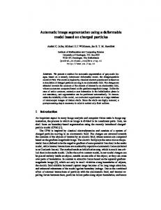
Given a set of training images together with their label maps, S = {(Yj , Xj ), j = (0) 1..m}: For each image Xj , construct probability maps Pj , with a distribution (possibly uniform) on all the labels. For t = 1, ..., T : (t−1)

• Make a training set St = {(yji , Xj (Ni ), Pj (Ni )), j = 1..m, i = 1..n}. • Train a classifier on both image and context features extracted from Xj (Ni ) and (t−1) Pj (Ni ) respectively. (t)

• Use the trained classifier to compute new classification maps Pj (i) for each training image Xj . The algorithm outputs a sequence of trained classifiers for p(n) (yi |X(Ni ), P(n−1) (Ni )) Fig. 1. The training procedures of the auto-context algorithm.

We can prove that at each iteration, ACM is decreasing the error t . If we note that the error of one example (i), at time t − 1 is P(t−1) (i)(yi ) and at time t is pt (yi |Xi , P(t−1) (i)), then we can use the log-likelihoods to formulate the error over all examples as in eqn. 2.

t−1 = −

P

i

log P(t−1) (i)(yi ), t = −

P

i

log p(t) (yi |Xi , P(t−1) (i))

(2)

First, it is trivial to choose p(t) to be a uniform distribution, making t = t−1 . However, boosting (or any other effective discriminative classifier) is guaranteed to choose weak learners to create p(t) that minimize t and will fail if none such exist, so therefore, if AdaBoost completes, t ≤ t−1 .

3

Results

3.1

Caudate Segmentation

We first tested our algorithm on a recently established caudate segmentation dataset [1]. 4 datasets were provided in this grand challenge competition, 2 for training and 2 for testing. As described in the documents from the organizers: “All MRI images are scanned with an Inversion Recovery Prepped Spoiled Grass sequence on a variety of scanners (GE, Siemens, Philips, mostly 1.5 Tesla). Some datasets have been acquired in axial direction, whereas others in coronal direction. All datasets have been re-oriented to axial RAI-orientation, but have not been aligned in any fashion.” Due to space limits, we refer the readers to [1] for definitions of the error metrics reported here. Results on the two test datasets were uploaded to the benchmark server; performance was measured by the benchmark test organizers. The first two rows are UNC pediatric and elderly datasets, and the third is from the Brigham Women’s Hospital.

Case UNC Ped UNC Eld BWH PNL Average All

OE 40.35 38.75 41.76 40.84

Score 74.62 75.63 73.73 74.31

VD -23.21 -17.23 -26.62 -23.93

Score 59.46 69.77 53.78 58.30

AD 0.86 0.75 1.51 1.22

Score 68.25 72.15 49.10 57.89

RMSD 1.21 1.14 3.50 2.53

Score 78.38 79.64 42.05 57.45

MD 5.64 6.79 25.27 17.33

Score 83.41 80.02 28.41 50.62

Total 72.82 75.44 49.42 59.71

Table 1. Error metrics on the caudate segmentation by [?]; and the overall score is 59.71. Case UNC Ped UNC Eld BWH PNL Average All

OE 33.42 36.79 32.07 33.34

Score 78.98 76.86 78.50 78.26

VD -12.05 -0.69 -13.62 -10.60

Score 76.50 80.04 74.42 76.03

AD 0.68 0.72 1.17 0.97

Score 74.76 73.37 76.55 75.51

RMSD 1.09 1.31 1.75 1.52

Score 80.47 76.53 76.45 77.31

MD 12.09 17.61 12.83 13.67

Score 64.44 48.21 62.26 59.78

Total 75.03 71.00 73.64 73.38

Table 2. Error metrics for caudate segmentation by the algorithm proposed here; the overall score is 73.38.

Given the ground truth segmentation (A) and an automated segmentation (B), along with d(a, b) defined as the Euclidean distance between 2 points, a and b, we define the following error metrics: • Precision = A∩B • H1 = maxa∈A (minb∈B (d(a, b))) B • Recall = A∩B • H2 = maxb∈B (mina∈A (d(b, a))) A 2 • Relative Overlap = A∩B • Hausdorff = H1 +H A∪B 2 • Similarity Index =

A∩B ) ( A+B 2

• Mean = avga∈A (minb∈B (d(a, b)))

Fig. 2. Error metrics used to validate hippocampal segmentations.

3.2

Hippocampal Segmentation

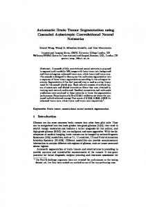
For a second test of our algorithm, we segmented the hippocampus in a dataset from a study of Alzheimer’s disease (AD) which significantly affects the morphology of the hippocampus [8]. This dataset includes 3D T1-weighted MRIs of individuals in three diagnostic groups: AD, mild cognitive impairment (MCI), and healthy elderly controls. All subjects were scanned on a 1.5 Tesla Siemens scanner, with a standard high-resolution spoiled gradient echo (SPGR) pulse sequence with a TR (repetition time) of 28 ms, TE (echo time) of 6 ms, field of view of 220mm, 256x192 matrix, and slice thickness of 1.5mm. For training we used 27 brain MRIs (9 AD, 9 MCI, and 9 healthy controls), and for testing we used an independent set of 83 brain MRIs (35 AD (age 77.40 ± 6.10), 22 MCI (age 72.27 ± 6.16), and 26 healthy controls (age 65.38 ± 8.35)). Prior to any training or testing, all subjects were registered using 9-parameter linear registration to a population mean template [9]. Fig. 3 shows a typical segmentation of the hippocampus after 0, 1, 4, and 10 iterations of ACM, compared with those of FreeSurfer. Zero iterations of ACM would be equivalent to traditional AdaBoost. Second, to assess segmentation performance quantitatively, we used a variety of error metrics, defined in Fig. 2. Training Precision Recall R.O. S.I. Hausdorff Mean

Left 0.914 0.868 0.802 0.890 2.96 0.00204

Right Testing Left 0.883 Precision 0.860 0.836 Recall 0.845 0.859 R.O. 0.739 0.857 S.I. 0.849 3.85 Hausdorff 3.68 0.00331 Mean 0.00411

Right FreeSurfer Left Right 0.857 Precision 0.587 0.588 0.750 Recall 0.878 0.917 0.656 R.O. 0.543 0.558 0.785 S.I. 0.700 0.713 4.61 Hausdorff 5.44 5.04 0.00370 Mean 0.432 0.271

Table 3. Precision, recall, relative overlap (R.O.), spatial index (S.I.), Hausdorff distance, and mean distance are reported for training and testing hippocampal segmentation after 10 iterations of ACM. FreeSurfer statistics are also reported for the same dataset for comparison. Distance measures are expressed in millimeters. A value of 1 is optimal for precision, recall, relative overlap, and similarity index; lower values are better for distance metrics.

Coronal

Axial

Left Sagittal

Right Sagittal

(a)

(b)

(c)

(d)

(e)

(f) Fig. 3. Hippocampal segmentations improve with the number of ACM iterations. (a) ground truth manual segmentation by an expert (b) 0 ACM iterations (c) 1 ACM iteration (d) 4 ACM iterations (e) 10 ACM iterations (f) FreeSurfer.

Training Precision Recall R.O. S.I. Hausdorff Mean

Left 28.90% 49.35% 74.95% 42.57% -69.53% -83.97%

Right Testing Left Right 10.92% Precision 36.08% 13.81% 35.89% Recall 42.12% 27.14% 42.82% R.O. 73.85% 34.66% 25.54% S.I. 43.22% 20.90% -45.82% Hausdorff -63.27% -39.13% -48.07% Mean -80.85% -52.75%

Table 4. Percent change is calculated for precision, recall, relative overlap (R.O.), spatial index (S.I.), Hausdorff distance, and mean distance of traditional AdaBoost (ACM with 0 iterations) and ACM with 10 iterations.

Table 3 summarizes the results through 10 iterations of ACM, and shows that, based on our metrics at least, it segments the hippocampus more accurately than FreeSurfer when using the standardized priors distributed with FreeSurfer. FreeSurfer tends to overestimate the size of the hippocampus as shown by the high recall, but lower precision. Our algorithm takes about 2 hours to train per iteration of ACM, but less than one minute to test (segment a new hippocampus) regardless of the number of ACM iterations, whereas FreeSurfer takes about 10-12 hours to segment a new brain. In fairness, FreeSurfer segments many hundreds of structures, but our algorithm, in this context, is only segmenting the hippocampus (although we could learn a model for any subcortical structure). Also, FreeSurfer is not given the opportunity to learn the specific nuances of this particular dataset, whereas our algorithm is trained on this dataset, which means that FreeSurfer’s segmentation could improve if it was given the opportunity to create an atlas based on this dataset. However, FreeSurfer is not provided with training options, and we used it in the standard way.

Hausdorff Distance

F‐value Hausdorff D Distance (mm)

0.95 0.9

f‐vvalue

0.85 0.8 0.75 0.7 0.65 0.6 0

1

2

3

4

5

6

7

8

9

10

11 10 9 8 7 6 5 4 3 2 0

1

Number of ACM Iterations Left Training

Right Training

Left Testing

2

3

4

5

6

7

8

9

Number of ACM Iterations

Right Testing

Left Training

Right Training

Left Testing

Right Testing

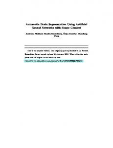
Fig. 4. Effects of varying the number of iterations of ACM on the Hausdorff distance, and the f-value, defined as the average of precision and recall. All error metrics tested in this paper improved as the number of ACM iterations increased.

To show the greatly increased power of using ACM versus just AdaBoost without ACM, Fig. 4 shows how two error metrics improve with the number of

10

iterations of ACM. Fig. 4 shows that ACM gives a large initial improvement, which levels off after about 4 iterations, in both the training and testing datasets, which shows that the AdaBoost learners at this point are relying too much on the features based on P(t−1) (Ni ) and not adding new informative features based P on X(Ni ). A stopping criterion can also be formulated, such as i (P(t) (i) − P(t−1) (i))2 <  (although this is not employed in this paper). Table 4 summarizes the added benefit of ACM, and shows an improvement in all metrics tested, especially the distance metrics and the relative overlap.

4

Conclusion

As shown using a variety of standard overlap metrics, ACM can improve the segmentation performance of AdaBoost for hippocampal and caudate delineation on MRI. ACM is applicable to a wide variety of imaging applications where the ROI is a connected shape. Such applications include detection of the cortical sulci, tumor recognition, and segmenting other subcortical structures; these applications will be the topic of future study. Additionally, ACM can be combined with any pattern recognition algorithm, not just AdaBoost, but AdaBoost allows easy incorporation of features based on P(t−1) .

References 1. van Ginneken, B., Heimann, T., Styner, M.: 3D Segmentation in the Clinic: A Grand Challenge. Proc. of MICCAI Workshop (2007) 2. Fischl, B., et al.: Whole brain segmentation: Automated labeling of neuroanatomical structures in the human brain. Neurotechnique 33 (2002) 341–355 3. Yang, J., Staib, L.H., Duncan, J.S.: Neighbor-constrained segmentation with level set based 3D deformable models. IEEE TMI 23(8) (August 2004) 940–948 4. Pohl, K., Fisher, J., Kikinis, R., Grimson, W., Wells, W.: A Bayesian model for joint segmentation and registration. NeuroImage 31(1) (2006) 228–239 5. Heckemann, R.A., Hajnal, J.V., Aljabar, P., Rueckert, D., Hammers, A.: Automatic anatomical brain MRI segmentation combining label propagation and decision fusion. Neuroimage 33(1) (October 2006) 115–126 6. Powell, S., Magnotta, V., Johnson, H., Jammalamadaka, V., Pierson, R., Andreasen, N.: Registration and machine learning based automated segmentation of subcortical and cerebellar brain structures. NeuroImage 39(1) (January 2008) 238–247 7. Oliva, A., Torralba, A.: The role of context in object recognition. Trends in Cognitive Sciences 11(12) (December 2007) 520–527 8. Becker, J., Davis, S., Hayashi, K., Meltzer, C., Lopez, O., Toga, A., Thompson, P.: 3D patterns of hippocampal atrophy in mild cognitive impairment. Archives of Neurology 63(1) (January 2006) 97–101 9. Collins, D., Neelin, P., Peters, T.M., Evans, A.C.: Automatic 3D intersubject registration of MR volumetric data in standardized Talairach space. J Comput Assist Tomogr 18 (1994) 192–205