in online route planning systems, with special focus on the fast computation of .... networks: less than one microsecond on a modern server. ...... path is particularly cheap in very local areas, since most shortcuts needed end up in cache. Query.
HLDB: Location-Based Services in Databases Ittai Abraham1 , Daniel Delling1 , Amos Fiat2 , Andrew V. Goldberg1 , and Renato F. Werneck1 1
2
Microsoft Research Silicon Valley School of Computer Science, Tel Aviv University. Visitor at MSR during this work June 2012 Technical Report MSR-TR-2012-59
This paper introduces HLDB, the first practical system that can answer exact spatial queries on continental road networks entirely within a database. HLDB is based on hub labels (HL), the fastest point-to-point algorithm for road networks, and its queries are implemented (quite naturally) in standard SQL. Within the database, HLDB answers exact distance queries and retrieves full shortest-path descriptions in real time, even on networks with tens of millions of vertices. The basic algorithm can be extended in a natural way (still in SQL) to answer much more sophisticated queries, such as finding the ten closest fast-food restaurants. We also introduce efficient new HL-based algorithms for even harder problems, such as best via point, ride sharing, and point of interest prediction. The HLDB framework makes it easy to implement these algorithms in SQL, enabling interactive applications on continental road networks.
Microsoft Research Microsoft Corporation One Microsoft Way Redmond, WA 98052 http://www.research.microsoft.com
1
Introduction
In the last two decades, GPS navigation and map-based services have been gaining sophistication and user base, with increasing digital map coverage and level of detail. This motivated research in online route planning systems, with special focus on the fast computation of shortest paths. These systems are usually highly specialized and separated from other online services. As many services are built on top of databases and developed by database programmers, implementing map-based services within databases is attractive. It would allow developers to leverage the power and expressiveness of a database language (such as SQL) to create new types of online services. The resulting systems would be easy to program, customize, and maintain. A natural approach to route planning is to use one of various speedup techniques for Dijkstra’s algorithm [15] recently developed by the algorithm engineering community (see [12] for a survey). Given a source s and a destination t, the fastest techniques can find the exact shortest path in a road network with tens of millions of vertices in a millisecond or less. This is achieved by preprocessing the network for a few minutes (or hours) to generate auxiliary data that speeds up queries. Any such technique can be implemented as an external distance oracle, a standalone module that runs outside the database but can be called from SQL to compute the distance or retrieve the shortest path between two points. In a recent survey [36], Sankaranarayanan and Samet argue that such an external oracle is not good enough, however. Instead, they propose to implement database distance oracles, which can be stored and queried completely in SQL, with no external calls. This would have several benefits. The database system automatically gives an external memory (and even distributed) implementation of the algorithm, enabling applications that use more information than fits in RAM. Having the preprocessed data directly in the database enables sophisticated queries (such as nearest neighbors) to be handled much more efficiently than making repeated calls to an external black-box distance oracle. Furthermore, additional constraints (such as “closest gas station open now”) can be naturally expressed in SQL. Although many such problems can be solved efficiently outside the database [9, 11, 12, 20, 28], external implementations are less portable, harder to maintain, and very difficult to customize. Unfortunately, translating any of the speedup techniques surveyed by Delling et al. [12] to SQL is hard. They rely on sophisticated data structures (such as graphs and priority queues) that cannot be implemented nearly as efficiently in databases [18]. The best previous database oracle we are aware of is due to Sankaranarayanan and Samet [35]. On a graph with n vertices, it can answer �-approximate queries in O(log n) time after a preprocessing stage requiring O(n�−2 ) space and Ω(n2 ) time. Their approach has two major shortcomings. First, the preprocessing requires computing Ω(n) shortest path trees, which takes quadratic total time. Using the techniques they suggest, this would take months on continental road networks, thus restricting the applicability of their algorithm to relatively small networks (fewer than a hundred thousand vertices). Second, it is approximate: the suggested driving route may deviate significantly from the optimum (by up to 10% in their most common scenario), or a query for five nearby restaurants may not return the closest one. If detected by users, even a few suboptimal outputs may undermine their confidence in the entire system. Exact solutions are clearly preferred. This paper closes the gap between external and database oracles by introducing HLDB, the first approach that enables exact location services for road networks of continental size in databases with no external calls. HLDB can answer spatial queries in real time, i.e., fast enough 1
s
t
Figure 1: Labeling algorithm: the hubs of s are circles, and those of t crosses. for interactive applications. HLDB is based on hub labels (HL) [1, 2, 3], a highly optimized version of a labeling algorithm [19, 8] tailored to road networks. HL is conceptually simple. During preprocessing, it creates distance labels associated with each vertex v in the network. A distance label for v consists of a subset of vertices (hubs), together with the distances between each of them and v. To find the distance from s to t, the query algorithm uses the fact that at least one vertex on the shortest s–t path must appear (as a hub) in the labels for both s and t. Figure 1 gives an example. Our main conceptual contribution is to show that distance labels (as opposed to arbitrary distance oracles) are a superior solution for implementing location services in databases. Distance labels allow exact point-to-point queries to be stated entirely in terms of set operations, which is not the case for arbitrary speedup techniques. HLDB queries can thus be implemented in a straightforward and efficient way using only relational database operators (SQL statements). Labels are also a natural fit to solve the well-known k closest points of interest (or k-nearest neighbors) problem [7]. In addition, we introduce new algorithmic techniques to efficiently implement even more sophisticated location services, such as k best via points (or k-path nearest neighbors), ride sharing, and point of interest prediction. Unlike any previous approach, the asymptotic running time of HLDB for these queries does not depend on the number of acceptable candidates (points of interest) in the system. Besides its flexibility, a crucial advantage of HLDB over previous database distance oracles is that it is exact—it always finds the shortest path, and not just approximations. Moreover, HLDB queries are very efficient, since they are based on HL, the fastest known external distance oracle algorithm for road networks. In short, HLDB is the first truly practical algorithm to handle exact location services within databases. It is efficient, with low preprocessing effort and real-time queries. It is portable and easy to use: with queries implemented entirely within the database, it can exploit the full expressive power of SQL. Finally, it is extensible: with the concepts of hubs and labels, it naturally supports sophisticated queries (beyond simple distance oracles) within the database with no loss in asymptotic performance. The remainder of this paper is organized as follows. Section 2 presents the background concepts on which HLDB builds. Section 3 introduces the basic setup, including label representation, pointto-point distance queries, and efficient approaches to store and retrieve the actual sequence of arcs on the shortest path. Section 4 shows how to extend the basic label-based approach to enable a rich set of spatial operations, including standard nearest neighbor queries (such as finding the closest restaurant), as well as more sophisticated ones (such as finding the best gas station on the way home that accepts credit cards). Finally, Section 5 presents detailed experimental evidence that our approach is indeed practical. Implemented in SQL within a standard relational database, HLDB queries run in milliseconds on continental road networks, and always find exact solutions.
2
1.1
Related Work
We now present a brief overview of the literature on distance oracles (both database and external) and related problems. Computing distances (finding shortest paths) on spatial networks is a classic problem. Dijkstra’s algorithm [15] can solve it in essentially linear time [23], but is still too slow for many applications on large networks. This has motivated the study of acceleration techniques, which use information gathered during a preprocessing stage to speed up queries. The traditional approach to database oracles is to use the associated geometric information (such as coordinates). Such techniques have indeed been the main focus of the database community [30, 34, 35, 37]. The most successful previous database oracle, due to Sankaranarayanan and Samet [35], is based on the observation that if two clusters of vertices are sufficiently far apart, then distances between pairs of points in different clusters are similar. By formalizing this observation, their oracle (pathDistance) can answer �-approximate queries in O(log n) time using O(n�−2 ) space. They also show how to use the oracle to implement more sophisticated queries, such as k-nearest neighbors. Building the oracle requires computing Ω(n) shortest path trees in the graph, in Ω(n2 ) total time. As a result, the oracle can only be evaluated on rather small instances (with fewer than 100 000 vertices, the size of a medium city). Combined with the fact that the oracle size is only practical for large �, this approach is not feasible for real-life applications on inputs of continental size. An advantage of this approach is that queries can be implemented entirely in SQL. If one is willing to use a graph to find point-to-point shortest paths (outside the database), one can obtain much better results [1, 2, 10, 12]. The best methods have fast preprocessing, low space overhead, and real-time queries. They can easily handle continental road networks with tens of millions of vertices, and find provably optimal shortest paths. Perhaps the most important speedup technique is sparsification, which uses the fact that road networks have strong hierarchies. Algorithms such as highway hierarchies (HH) [32], contraction hierarchies (CH) [22], and reach-based routing (RE) [25] run a bidirectional version of Dijkstra’s algorithm, but prune unimportant vertices as the searches move farther from the source and the target. To ensure optimality, the preprocessing stage measures the importance of each vertex according to a mathematical definition. Another speedup technique is transit node routing (TNR) [4]. During preprocessing, it computes a large table with the distances between the most important vertices in the graph, enabling long-range queries to be answered with a few table lookups. Local queries must still use a standard Dijkstra-based algorithm, such as CH. By combining sparsification with goal-direction techniques (such as A∗ search [24] or arc flags [26]), which guide the search towards the target using information gathered during preprocessing, further speedups are possible [5, 25]. Many of these techniques perform well in practice and found their way into production systems, but no theoretical justification for their good performance was known. Recently, Abraham et al. [3] proved that variants of CH and RE have sublinear query bounds on graphs (such as road networks) with small highway dimension, a new concept they introduced. They showed even better bounds for a labeling algorithm [19]. Two follow-up papers [1, 2] introduced HL, a practical implementation of the labeling algorithm that has the fastest known queries on continental road networks: less than one microsecond on a modern server. Other approaches offer different trade-offs between preprocessing time, space usage, and query times. In fact, several algorithms (including TNR, CH, arc flags, HH, RE, and CRP [10], which is
3
partition-based) are fast enough to implement external distance oracles, answering exact queries in a few milliseconds (or less) on continental road networks. Besides having the fastest queries, this paper shows that HL has a crucial advantage for database applications: its query is a simple set operation (pick the minimum element in the intersection of two sets), and can be naturally expressed in SQL. All other algorithms need more complicated logic and data structures (even TNR, because of local queries), which makes it hard to use them as database oracles. Extended query scenarios, like finding the k-closest points of interest (or neighbors) to a vertex or to a whole path, have motivated extensive research in the database community [6, 7, 27, 30, 34], but these techniques are either approximate or only applicable to small road networks (or both). Many of these applications have external (non-SQL) solutions [20] based on the fast computation of of one-to-all [9], one-to-many [11], and many-to-many [28] shortest paths. One of our contributions is to show how to incorporate (and extend) these ideas within HLDB, enabling their use with SQL.
2
Background
This section introduces definitions and notation used in the rest of the paper. The point-to-point shortest path problem takes as input a directed graph G = (V, A), with a nonnegative length function `(v, w) associated to each arc (v, w) ∈ A. Given a source s and a target t, we must find the length dist(s, t) of the shortest path in G from s to t. A well-known solution is Dijkstra’s algorithm [15], which processes vertices in increasing order of distance from s, and stops when t is reached. With the appropriate priority queues, the algorithm runs in essentially linear time not only in theory [16, 14] but also in practice: it is only two to three times slower than a simple breadth-first search [23]. One can save time by running a bidirectional version of the algorithm. We focus on road networks, where vertices represent intersections, arcs represent road segments, and lengths correspond to travel times. As a running example, we use a real-world [31] representation of the road network of (Western) Europe with 18.0 million vertices and 42.2 million arcs, made available for the 9th DIMACS Implementation Challenge [13]. On road networks, bidirectional Dijkstra visits a significant fraction of the entire graph on long-range queries, which takes seconds even with a fully optimized in-memory implementation [9], too much for interactive applications. On road networks, two-phase algorithms can solve the point-to-point problem much more efficiently. The preprocessing phase takes only the graph as input and produces a moderate amount of auxiliary data. Efficient methods typically take minutes or hours on continental road networks. The subsequent query phase answers queries in on-line fashion, taking a source s and a target t as inputs and using the auxiliary data to find the shortest s–t path. In particular, our approach is based on the hub labels (HL) method. HL is a labeling algorithm [19]: for each vertex v in the graph, it builds a forward label Lf (v) and a reverse label Lr (v). The forward label Lf (v) consists of a sequence of pairs (u, dist(v, u)), where u is a vertex (a hub in this context). Similarly, Lr (v) consists of pairs (u, dist(u, v)). Note that the hubs in the forward and reverse labels of v may differ. Collectively, the labels obey the cover property: for any two vertices s and t, Lf (s) ∩ Lr (t) contains at least one vertex on the shortest s–t path. Given this property, an s–t query is trivial: among all vertices u ∈ Lf (s) ∩ Lr (t) (each of which defines a valid s–t path), pick the one minimizing dist(s, u) + dist(u, t) and return this sum. If the entries in each label are sorted by hub ID, this can be done with a coordinated sweep over 4
Algorithm 1: sql dist Input: source s ∈ V , target t ∈ V 1 2 3 4 5 6 7
SELECT MIN(forward.dist+backward.dist) FROM forward,backward WHERE forward.node = s AND backward.node = t AND forward.hub = backward.hub
the two labels, as in mergesort. Abraham et al. [3] showed that, on road networks, one can pick labels that ensure polylogarithmic point-to-point query times. This result is mostly theoretical: it relies on a preprocessing routine that, although polynomial-time, is impractical for continental road networks. More recently, Abraham et al. [1, 2] proposed HL as a practical implementation of the labeling algorithm. They show that one can construct labels if an ordering of the vertices is given. For road networks, the most efficient approach is to recursively compute labels according to the ordering: at each step, it picks the next vertex v in the order and shortcuts it. To shortcut v, we remove it from the graph and add shortcut arcs between its neighbors as necessary to preserve distances between them [22]. (Note that each shortcut is built from two other arcs/shortcuts.) After shortcutting v, the algorithm recursively computes the labels in the remaining graph, then computes v’s label from those of its neighbors. We denote by A+ the set of shortcut arcs added during this process. The average label size depends on the ordering. Abraham et al. [2] study efficient methods to find good orderings. The fastest method uses the ordering computed by CH preprocessing, which considers vertices bottom-up (from least to most important). Ordering vertices top-down is slower, but yields smaller labels, with fewer than 80 hubs on average on Europe. Both methods can be combined for different trade-offs. In this paper, we assume the labels are given, and focus on how to use them efficiently within the database.
3
Point-to-Point Shortest Paths
We are now ready to explain how HL queries can be naturally expressed in SQL. By storing all labels in a database, we can run pure SQL code to obtain not only the distance between any two points, but also a description of the corresponding shortest path.
3.1
Distance Queries
We store the labels in two tables, forward and backward. Each table contains all labels of the corresponding direction, and has three columns: node, hub, and dist. For each vertex v, we store entries (u, dist(v, u)) ∈ Lf (v) as triples (v, u, dist(v, u)) in forward. Similarly, backward stores a triple (v, u, dist(u, v)) for each (u, dist(u, v)) ∈ Lb (v). To determine the distance between a source s and a target t, we just have to find the shared hub of the source’s entries in forward and the target’s entries in backward that minimizes the sum
5
of the forward and backward distances. The corresponding SQL statement is given in Algorithm 1. Since the number of rows in forward and backward is huge (about 1.35 billion each on Europe), we need appropriate indices. Algorithm 1 needs fast access to the rows of source and target (lines 5 and 6), followed by fast access to specific hub entries (line 7) within these rows. We thus build a composite clustered index on node (primary) and hub (secondary). All rows corresponding to the same label are stored together to minimize random accesses to the database.
3.2
Path Retrieval
Algorithm 1 computes only the distance between any two vertices s and t in the network. We now show how to retrieve the actual list of arcs (or vertices) on the shortest s–t path P , which may be needed for some applications. The simplest approach is to retrieve the path one arc (or vertex) at a time [4]. For example, an s–t query could return not only dist(s, t), but also the first arc (s, v) on the s–t path. One can then retrieve the full path by performing multiple queries. Shortcut-based methods [22, 25] often use a faster two-stage approach. They first find the shortest s–t path P + in G+ . The path consists of very few shortcuts (around 20 for Europe). Then they repeatedly use a precomputed map to translate each shortcut into its two constituent shortcuts (or arcs). Eventually, only original arcs are left. Unfortunately, this approach would still be too slow for HLDB, since retrieving a single shortest path could require thousands of non-sequential accesses (up to one for each arc on the path). We could avoid non-sequential accesses by simply storing in the database the full description (sequence of arcs) of the shortest paths between every node and each of its hubs. If an s–t query meets at a hub v, we could just concatenate the (precomputed) s–v and v–t paths to obtain the shortest path. The space requirements are prohibitive, however: on Europe, these paths have close to one trillion arcs in total. We opt for an intermediate approach: we actually store preassembled subpaths. During preprocessing, we store the full sequence of arcs for each shortcut in the graph. Queries then work in two stages: first find the shortest s–t path P + in G+ , then translate each shortcut in P + into the corresponding arcs. This approach requires only O(|P + |) random accesses, and was first proposed by Sanders et al. [33] in the context of an external memory implementation of CH. To support path retrieval within HLDB, we store additional precomputed information in the database. We assign a unique arc ID to every original arc, and a unique shortcut ID to every arc of A ∪ A+ . Note that each original arc has both an arc ID and a shortcut ID, and they are not necessarily the same. Shortcuts (and their IDs) are internal to the algorithm, whereas arc IDs can be set by the user. To translate each shortcut into its arcs, we keep a table called shortcuts. It has three columns (sid, aid, aseq), meaning that aid is the aseq-th arc on shortcut sid. A shortcut has one row in shortcuts for each arc it contains (in order). We also need additional fields in each label entry. We add extra columns to forward (besides node, hub, and dist): phub represents the parent hub (the predecessor of hub on the path from node in G+ ), and sid is the ID of the shortcut (or arc) from phub to hub. We augment backward in a similar way: phub represents the successor of hub on the path to node in G+ , and sid represents the shortcut (or arc) from hub to phub. In both tables, we set phub and hub to an invalid ID (−1) for rows where hub = node. An s–t query can then be implemented in three stages.
6
First, we run a query similar to Algorithm 1. Instead of finding just the s–t distance, it must also return the meeting hub of the s–t path, together with the phub and sid fields in the corresponding rows of forward and backward. The second stage builds a temporary table spath with the sequence of shortcuts on the s–t path P + . Each row has two columns: sid represents a shortcut, and sseq is an integer indicating the relative order of this shortcut within P + . If shortcut sa appears before sb in P + , the row representing sa must have a lower sseq than the row representing sb . We build spath one row at a time. Suppose x is the hub responsible for the s–t path. First, we add to spath the shortcuts on the subpath of P + between s and x by following parent pointers in Lf (v), represented by phub and sid in forward. (This can be done in SQL with a WHILE loop.) Since this will give shortcuts in reverse order, we assign decreasing sseq values to them: −1, −2, −3, . . . We then do the same for the shortcuts in the subpath of P + between x and t. Since now parent pointers give us shortcuts in the right order, we just assign increasing sseq values to the shortcuts we find: 1, 2, 3, . . . Note that shortcuts in the x–t subpath have higher sseq than shortcuts in the s–x subpath. The third stage of the algorithm expands each shortcut in P + into the corresponding sequence of arcs. It does so by joining spath and shortcuts on column sid, ordering the resulting rows by sseq and aseq. The final table contains the IDs of all arcs on the shortest s–t path in order.
4
Extended Scenarios
So far, we have considered how to implement a distance oracle directly in SQL. This section shows how to use labels to answer more sophisticated queries more efficiently than using only a distance oracle. The problems we consider need all or some distances to a subset of vertices P (the POIs). The simplest such location services (like finding the k closest POIs) depend only on a query source and a set of previously known POIs. As Section 4.1 will show, we can solve these problems efficiently by extracting the POI labels in advance and indexing them by their hubs. Many other natural location services are not as simple, however, since they also depend on a query target. An obvious example is finding the best post office on the way home, i.e., the one yielding the smallest detour; other problems, such as ride sharing and POI prediction, have similar properties. Section 4.2 introduces new algorithmic techniques to handle such scenarios efficiently and shows how they translate to HLDB.
4.1
Single-Hub Indexing
Consider the scenario where many queries (from different sources) are to be made using the same set of points of interest. An obvious example is the “store locator” feature of many web sites: users need the closest Starbucks or the three closest Citibank ATMs. Formally, we must find the k closest POIs to a source s. The straightforward solution is to compute the distance from s to all POIs with an external distance oracle, and report the closest. With this approach, queries take time linear in |P|. Previous work [30] suggests filtering the POIs (typically by Euclidean distance), but this may lead to suboptimal results and complicates the query. With labels in the database, one can do better. As Figure 2 shows, each shortest path from s to a POI must pass through one of the hubs of s. So we can find the k closest POIs for each hub of s and then pick (among those) the k closest overall. To implement this efficiently, we use 7
Algorithm 2: sql k poi dist Input: source s ∈ V , number k 1 2 3 4 5 6 7 8 9
SELECT TOP k MIN(forward.dist+poilab.dist) AS dist, poilab.node FROM forward,poilab WHERE forward.node = s AND forward.hub = poilab.hub GROUP BY poilab.node ORDER BY dist
a preprocessing step to extract from backward a table poilab with only the relevant rows—those where node corresponds to a POI. This can be done using a JOIN with the table representing the POIs. Next, we build a clustered index on hub and dist (including node for performance). We can now run queries using poilab instead of backward, as shown in Algorithm 2. Note that there are only minor differences relative to Algorithm 1 (besides the use of poilab). We return k distances, each with the POI responsible for it. We also need the GROUP BY operator to make sure we only consider the best hub for each potential POI. Without it, we could return multiple paths to the same POI (using different hubs). Also note that the number of random accesses to the database is bounded by |Lf (s)|, not |P|. This simple query algorithm does not exploit the fact that we only need to look at k POIs per hub—it will actually scan all POIs that share a hub with s. Because the most important vertex in the graph is a hub for all other vertices, the running time still linear in |P|. We can remedy this with a slightly more complicated query algorithm: we use a cursor to iterate over all hubs of the source and determine the k closest vertices for each hub. Since poilab is indexed by hub and dist and labels are small, this is faster than the straightforward approach when there are many POIs. We can still restrict the set of acceptable POIs (by opening hours, for example) using a WHERE clause when determining the closest k POIs of a hub. When k is known in advance and no further constraints apply (all POIs are acceptable), we can use a tailored version for even better performance. When building poilab, we only need to keep the k rows with the smallest dist values for each distinct hub h. Additional rows cannot possibly be part of the final solution for any source s: among paths that use h, the first k entries dominate the others. If k is small relative to the number of POIs, we can use Algorithm 2 to query the k closest POIs. As experiments will show, this approach is faster, mainly because we do not use a cursor. Moreover, since the number of rows per hub is now limited by k, the total p1
p3 p2
p4
s
p5
Figure 2: Finding the closest POI: the hubs of s are circles, those of the point of interests crosses.
8
running time is still linear in k, and not |P|. Additional improvements are possible for k = 1, when we need to find only the closest POI. Because each hub appears at most once in poilab, we can make it a primary key, eliminating the need for a clustered index and for the GROUP BY operator. In this case, one can think of poilab as a superlabel : this is the label one would obtain if all points of interest were conflated into a single vertex. In essence, this hub indexing strategy is a translation into SQL of the bucked-based approach [28]: it creates a separate bucket for each hub in the (potentially large) target set, but queries only need to access buckets that represent hubs in the (much smaller) forward label. This approach was originally developed to solve the one-to-many problem: computing the shortest path from s to each element of a predefined set of targets (points of interest). Geisberger [11] has recently shown that this approach can be used (as an extension of CH) to solve the k-closest POI problem efficiently.
4.2
Double-Hub Indexing
For location services that depend on a query source s, a query target t, and a set of predefined POIs P, single-hub indexing is not good enough. For example, consider the best via point problem [6, 30, 11]: assume you want to go from s to t but need to stop at a post office on the way while minimizing your overall travel time. Formally, you want the post office p that minimizes dist(s, p) + dist(p, t). Again, the straightforward approach is to run two external distance oracle queries (from s and to t) for each via point and report the one with the minimum sum. This yields a running time linear in |P|, the number of candidate via points. We can do better in practice with single-hub indexing. We build two tables vialabF and vialabB containing the relevant POI rows of forward and backward, indexed by hub and dist. To find the best via point for a given source s and target t, we compute the distances from s to all POIs and the distances from all POIs to t. We return the POI that minimizes the sum of both distances. Unfortunately, the running time of this approach is still linear in |P|, since we must consider all acceptable via points. We now propose a new approach, called double-hub indexing, which is asymptotically faster when |P| is large. Every path we are interested in is the concatenation of two shortest paths: from s to a POI p, then from the same POI p to t. We need to find the POI p such that the total length is minimized, but without testing all candidates POIs explicitly. Let h be the meeting hub for path s–p and h0 the meeting hub for p–t. Note that h is a forward hub for s and h0 is a backward hub for t; most importantly, both h and h0 are hubs of p (reverse and forward, respectively). For a given s–t via query, therefore, it suffices to look at all pairs (h, h0 ) such that h is a forward hub for s and h0 a reverse hub for t. To do so efficiently, we precompute (before queries) the POI
p2
t
s p1
p3
Figure 3: Best via point: forward hubs are circles, backward hubs are crosses; distances from incoming to outgoing hubs for each POI are precomputed.
9
p∗ for which dist(h, p∗ ) + dist(p∗ , h0 ) is minimized (among all POIs that have both h and h0 as reverse and forward hubs, respectively). Figure 3 gives an example. We can implement this idea in HLDB as follows. For the set of all POIs (via points), we build a table called vialab with four columns: node, hubF, hubB, and dist. For each POI (node) p, we store |Lb (p)| · |Lf (p)| rows. For each combination (hb , hf ) of backward and forward hubs of p, we store hf in hubF, hb in hubB, and dist(hb , p) + dist(p, hf ) in dist. We index vialab with a clustered index by hubF, hubB, and dist (including node for performance). Given s and t, the query algorithm now invokes two cursors looping over all combinations of hubs hf ∈ Lf (s) and hb ∈ Lb (t). For each pair of hubs, we access vialab and find the best via point p for this pair. We store p, together with dist(s, p) + dist(p, t) (obtained from vialab.dist, forward.dist, and backward.dist) in a temporary table temp. In the end, we return the row from temp with minimum distance. With this double-hub indexing approach, query times depend on the square of the sizes of the labels, which can be considerably smaller than |P|. This approach can easily be extended to the k best via nodes (and not just one). In the inner loop, we return (and store in temp) the k best via points for the particular pair of hubs. Then, we return the best k rows from temp with the additional constraint that we group the result by the via point. The running time still depends on k and the square of the size of the labels, but not on the number of POIs. 4.2.1
Ride Sharing
The ride sharing problem [21] can also be solved with our double-hub indexing approach. The goal is to match queries (people looking for a ride from an origin s to a destination t) to offers (drivers offering rides with origin s0 and destination t0 ). Given a new query (s, t), the goal is to find the offer (s0 , t0 ) that minimizes the (absolute) detour for the driver, given by dist(s0 , s) + dist(s, t) + dist(t, t0 ) − dist(s0 , t0 ). We are interested in an on-line solution: new queries are immediately matched with current offers whenever possible. To solve this with HLDB, we store all offers in a table offers with four columns: id (a unique offer identifier), source (the source vertex), target (the target vertex), and dist (the distance between source and target). Note that we can compute the distance when we feed a new offer into offers. As in the via point application, we then build a table offlab similar to vialab, with four columns: id, hubF, hubB, and dist. For each offer (s0 , t0 ), we store for each combination hf ∈ Lf (s0 ), hb ∈ Lb (t0 ) the offer’s identifier in id, hf in hubF, hb in hubB, and dist(s0 , hf ) + dist(hb , t0 ) − dist(s0 , t0 ) in dist. The query algorithm for a pair (s, t) works as in the via node problem, with two cursors looping over each combination hb ∈ Lb (s), hf ∈ Lf (t). Again, query times depend only on the number of hubs in s and t. This is better than in the approach proposed by Geisberger et al. [21], whose query times depend heavily on the number of available offers. 4.2.2
POI Prediction
Another application of double-hub indexing is POI prediction. Often a user knows her way and does not enter a destination into her navigation system. While driving, however, she may decide to stop for gas (or another service). Intuitively, if she asks the system for a nearby gas station, the best answer may not be the closest one, since it could actually be behind the user. This motivates
10
the need for POI prediction, i.e., reporting a reasonable POI that is “ahead” of the user, even if her final destination is unknown. Formally, we consider the following problem. Suppose the user is at vertex v, and has traveled for some time on a shortest u–v path (which has been tracked by the system), and asks for k POIs that are close and “on the way”. We propose finding POIs that are close to v (closeness criterion) and such that the path from u to the POI via v is not much longer than the shortest path from u to the POI (detour criterion). To achieve this, we assign a score S(p) = dist(u, v) + (1 + �)dist(v, p) − dist(u, p) to each POI, and report the k POIs with the smallest S(p) values. One can interpret S(p) as the sum of two terms. The dist(u, v) + dist(v, p) − dist(u, p) term is the length of the detour one makes by going from u to p through v. The � · dist(v, p) term is proportional to the distance from v to p. The value of � is chosen to achieve the desired balance between detour length and closeness and may vary with the type of POI. For example, closeness is more important for finding the nearest restroom than the nearest post office, so in the former case � is bigger. A straightforward implementation computes S(·) for all POIs and has running time linear in |P|. If � is predefined (experiments indicate that 0.05 is a reasonable value), double-hub indexing gives a more efficient solution. First, note that we can remove dist(u, v) from S(p), since it is the same for all POIs. So we need to evaluate (1 + �)dist(v, p) − dist(u, p) for each POI p. To do so efficiently, we use a preprocessing stage to build a table predlab with four columns: node, hub, hubprime, and dif. For each POI (node) p, we store |Lf (p)| · |Lf (p)| rows in predlab; more precisely, for each combination (h, h0 ) of backward hubs of p, we store h in hub, h0 in hubprime, and (1 + �)dist(h, p) − dist(h0 , p) in dif. An (u, v) query then works as in the best via point algorithm. For each pair of hubs h ∈ Lf (u) and h0 ∈ Lf (v), we use predlab to find the best POI for (h, h0 ), then pick (among those) the one minimizing S(·). Note that we can use any other ranking function that depends only on the lengths of the paths between u, v, and p. The fastest previous methods for POI prediction [29, 17] first compute a probability distribution of all possible user destinations, then rank POIs accordingly. By ranking POIs directly, our approach can be much faster.
5
Experiments
We now present a detailed evaluation of our approach. To the best of our knowledge, no previous practical algorithm has actually been evaluated within a database; for fairness, Section 5.1 compares existing methods with a standalone version of HL. Section 5.2 then considers full-fledged HLDB, with queries implemented entirely within the database. All experiments were run on a machine with two Intel Xeon X5680 CPUs and 96 GB of DDR3-1333 RAM, running Windows Server 2008 R2. Our main benchmark instance, representing Western Europe, has 18.0 million vertices and 42.2 million arcs. We also tested a moderate-sized instance representing Florida, with 1.07 million vertices and 2.71 million arcs. Both graphs were made available for the 9th DIMACS Implementation Challenge [13]. Other road networks, including proprietary ones, led to similar results. Our implementation of label generation is the same as in Abraham et al. [2]. It is implemented in C++ using Visual Studio 2010, with OpenMP used for parallelization.
11
method SILC PCP pathDis pathDis CH HL-0 HL-17 HL-∞
src. [34] [37] [35] [35] [22] [2] [2] [2]
input size |V | 4k 60k 90k 90k 18M 18M 18M 18M
preprocessing time space [s] [b/v] n.a. > 10 n.a. 100 n.a. 75 n.a. 30000 143 23 181 1344 1188 1075 20580 998
query time error [ns] [%] > 1 000 000 > 0 35 000 20 68 000 10 > 100 000 1 78 706 — 700 — 545 — 508 —
Table 1: Performance of C++ implementations of various distances oracles.
5.1
C++ Implementation
Table 1 summarizes the performance of standalone C++ implementations (outside the database context) of contraction hierarchies (CH) [22] and a few HL variants [2], which use various combinations of top-down and bottom-up ordering to achieve different trade-offs between preprocessing time and label size. HL-0 uses pure bottom-up ordering, HL-17 orders the 131 072 most important vertices top-down and the rest bottom-up, while HL-∞ approximates a top-down ordering for all vertices. For comparison, we also give the numbers reported by Samet et al. for various distance oracles [34, 37, 35] (which only work on small problems). Their implementations are also in C++, and the machine they use is less than twice as slow as ours. For each algorithm, we show the number of vertices on the graph on which it was tested, the preprocessing time (in seconds), the total space usage (in bytes per vertex), the average sequential time for random queries, and (for approximate oracles) the maximum allowed percent error. While HL-0 and HL-17 preprocessing takes only a few minutes for Europe. Samet et al. preprocessing is very slow and practical only for small graphs. They do not report preprocessing times, but among other things their preprocessing uses Dijkstra’s algorithm to build n shortest path trees. On Europe, a state-of-the-art implementation would take months to build the trees [9]. A recent algorithm [9] can build the trees much faster on a high-end GPU, but it is unclear if it can be augmented to efficiently perform the additional work of the preprocessing algorithm. Even if it could, preprocessing on Europe would take days. We observe that both CH and HL are clearly superior solutions when used as external distance oracles. They can handle much bigger graphs, preprocessing space can be much lower, and queries are faster and provably exact. HL is two orders of magnitude faster than the oracles by Samet et al. even on graphs more than two orders of magnitude bigger. CH is slower than HL, but it can still answer queries in less than 100 µs, which is fast enough for real-time applications. Moreover, CH requires much less RAM than HL; because it uses a graph for queries, however, it cannot be implemented efficiently within the database. The values in Table 1 are for distance-only queries. To support path unpacking, HL needs 11 more seconds of preprocessing, and an extra 1.2 GB for maintaining full descriptions of all shortcuts. With parent pointers, the total space usage increases from 18.0 GB to 29.4 GB. With the additional data, HL can retrieve the full path in about 5 µs. CH queries have similar additive increases using preassembled shortcuts (which requires an extra 1.2 GB of data). 12
5.2
Database Queries
We now evaluate our approach within a database system. We implemented HLDB queries in SQL using Microsoft SQL Server 2008 R2 (limited to 8 GB of RAM). The database files are stored on a RAID-0 of two Intel 320 SSD drives with 160 GB each. To evaluate queries, we ran a C++ program on the same machine, calling the SQL server via ODBC. We measured the time from requesting a query to the SQL server to getting an answer from it. We inserted the labels of HL-17 for Europe (with 75.0 hubs on average) into the database ordered by node and then hub, producing tables (forward and backward) with roughly 1.35 billion rows taking 36.8 GB each (including parent information and indices). The table with precomputed sequences of arcs (shortcuts) has 205 million rows and takes 5.1 GB. The total space usage is therefore 78.8 GB. This is more than the almost 30 GB used by the C++ implementation of HL, which represents labels more compactly. For Florida, we ran HL-14 (top 16 384 vertices ordered top-down) preprocessing, which takes 28 seconds. The resulting labels have 38.8 hubs on average, and take about 41.5 million rows (1.14 GB) per direction in the database. The shortcuts table has 12.7 million rows and 319 MB. We always clear the DB cache before each experiment, and by default store the database on SSD. To compare internal HLDB queries with external calls to an HL-based distance oracle, we implemented the latter in C#, which can be called from MS SQL. Compared to the C++ implementation, the C# version is slower by roughly a factor of 2.5 (random distance queries on Europe take 1335 ns on average), partially because our C# implementation is less optimized. 5.2.1
Random Queries
In our first experiment, we ran one million point-to-point queries, with the source s and the target t picked uniformly at random among all vertices in the graph. We ran three variants of our SQL query: computing only the s–t distance, retrieving the compact path P + (the path with shortcuts), and retrieving the full path. Each variant does strictly more work than the previous one. We also evaluated our external C# distance oracle, kept entirely in RAM and outside the database. Figure 4 shows the average time of the first q queries in Europe, with q varying from 10 to 1 000 000. Average times decrease as more SQL queries are processed, since more information is gradually brought to RAM. In particular, the distance-only variant needs 3.27 ms per query for the first 10 queries, but one million queries take 1.97 ms on average. The variant that finds the full path benefits the most (since it makes more random accesses), with times decreasing from 23.7 ms to 8.7 ms. Results are even better on smaller instances. As shown in Figure 5, queries on Florida are about twice as fast as on Europe. Note that all variants of HLDB are fast even with cold cache. Retrieving each of the first 10 paths takes less than 25 ms on average on Europe, which is good enough for interactive applications. Comparing the performance of the SQL query to the external oracle (which resides in memory), we observe that the difference in performance is relatively small. For the C# implementation of HL, most of the 0.6 ms of the query time is due to overhead for making an external call from MS SQL Server.
13
●
10
● ●
●
+ x
+ x
105
106
101
102
+ x
+ x
0
+ x
5
+ x
25 15
●
0
query time [ms] 5 10 15 20
+ x
path retrieval compact path distance only external
20
25
●
●
103 104 number of queries
Figure 4: Average HLDB times on Europe for random point-to-point queries (SSD).
+ x
10
●
path retrieval compact path distance only external
15
●
●
5
●
+
●
101
102
+ x
+ x
●
+ x
+ x
105
106
0
x
+ x
0
query time [ms] 5 10
15
●
103 104 number of queries
Figure 5: Average HLDB times on Florida for random point-to-point queries (SSD).
14
10
●
●
8
+ x
query time [ms] 4 6 8
●
6
●
●
● ●
2
●
+ x
+ x
+ x
+ x
+ x
+ x
+ x
+ x
+ x
+ x
+ x
0
+● x
●
+ x
0
+● x
●
●
+ x
4
● ●
2
10
path retrieval compact path distance only external
●
210
212
214
216 218 ball size
220
222
224
Figure 6: Average times on Europe for 10 000 local queries (SSD). 5.2.2
Local Queries
Picking source and target at random produces mostly long-range queries, but typical users are interested in local queries, which should be faster. We simulate such queries by preselecting s–t pairs as follows. Given a ball size b, we first pick a vertex x at random, run Dijkstra’s algorithm from x until b vertices are scanned, then pick sources and targets uniformly at random among the scanned vertices. Figure 6 shows the average query times on Europe for all three variants of HLDB as a function of b. For each ball, we run 10 000 queries from a cold start; each point in the plot is the average of 10 balls of the same size. As expected, all types of queries are faster in more restricted regions. Reporting the entire path is particularly cheap in very local areas, since most shortcuts needed end up in cache. Query locality also has some effect on distance and compact path queries, but it is not as pronounced. 5.2.3
Single-Hub Indexing
We now consider more complex scenarios, starting with point of interest (POI) queries. Given k, a source s, and a set of POIs P, we must find the k closest POIs from s, as well as the corresponding distances. Recall that Section 4.1 considered three algorithms to solve this problem: the straightforward approach using an external oracle, the general approach using a cursor to iterate over all the hubs of s, and a tailored version where k must be preselected. Figure 7 shows how these algorithms perform on Europe for k = 1 and k = 16 as a function of |P|. We pick a set of POIs uniformly at random from the entire graph, then run 10 000 queries (from cold cache) from random sources. Each point is an average taken over 10 sets of POIs.
15
100
x
x ●
●
●
●
●
●
●
●
●
x + +● +● +● +● +● +● + + + + + + + + + + + + x x x x x x x x x x x x ●
●
●
0.1
●
10
x
0.1
query time [ms] 1 10
+ x
x
k = 16 (T) k = 1 (T)
k = 16 (C) k = 1 (C) external oracle
1
100
●
20
22
24
26
28 210 212 number of POIs
214
216
218
Figure 7: Time to find the closest POI as a function of the number of POIs (10 000 queries, SSD). Since the times of the oracle-based approach are essentially independent of k, we only report them once. We observe that the oracle-based approach depends heavily on |P|. Initially, running times are dominated by the overhead of the external calls; eventually, doubling |P| doubles the running time as well. For large |P|, the algorithm is too slow for interactive applications. In contrast, our SQL-based algorithms show little dependence on |P|. The impact of k is also limited: the cursor-based version (C) is less than twice as slow for k = 16 than for k = 1. The tailored query (T) is up to three times faster, but not as flexible as the cursor-based version, which allows additional constraints. All SQL-based algorithms take less than 8 ms for all scenarios considered, fast enough for online applications. Note that both curves for the tailored SQL query follow the same pattern: running times increase with the number of POIs, decrease abruptly, then start increasing again. These results indicate that the system uses heuristics to decide which strategy to use for intersecting Lf (s) and the (usually larger) table representing the POIs. Initially, it traverses the label and poilab in full (with running time linear in |P|). When there are enough POIs, it performs multiple searches in the POI table, looking only for hubs that appear in Lf (s) (running time logarithmic in |P|). Sankaranarayanan and Samet report query times for k-closest POIs as well (Figure 18(a) in [35]). On a road network with 91 113 vertices (much smaller than ours), they pick 911 random vertices as POIs. Queries are fast for k = 1 but take more than 1 ms for k > 10, even though they are implemented in C++ (with no database involved) and are approximate. We obtain comparable results with an exact algorithm implemented in SQL (which is much slower than native C++) and on an input that is 200 times as large.
16
1000 ●
x● ● +● + + + + +● +● +● +● +● +● +● + + + + + x ●
●
●
●
●
100
●
+● +●
300
x
30
x x DC: (k = 16) DC: (k = 1) all−POIs
●
+ x
3
x x x x x x x
10
x x
3
10
query time [ms] 30 100 300
1000
x
20
22
24
26
28 210 212 number of POIs
214
216
218
Figure 8: Time to find the best via point as a function of the number of POIs (1 000 queries, SSD). 5.2.4
Double-Hub Indexing
We study the performance of HLDB on location services requiring double-hub indexing. For simplicity, we focus on k best via point queries; ride sharing and POI prediction have similar behavior. We evaluate two algorithms, one based on two cursors (DC) and another that evaluates the distances from s to all POIs and from all POIs to t (all-POIs). As before, we pick a varying number |P| of random POIs from the graph and evaluate the performance of both algorithms for k = 1 and k = 16. We run 1 000 queries from cold cache from random sources. Figure 8 gives the results. As expected, the all-POIs approach becomes too slow as |P| increases. (Since its running time is the same for both values of k, we only report k = 1 in the figure.) In contrast, the running time of the double cursor approach increases only slightly with |P| (by a factor of three when |P| increases from 1 to 262 144), mainly due to the fact that a larger fraction of the pairs of hubs determined by s and t end up having entries in vialab. With running times below 420 ms even for a large number of POIs in the system, the approach is still fast enough for practical applications. 5.2.5
Impact of the SSD
We now evaluate HLDB when, instead of using SSDs, we store files on two Seagate Constellation 7200 SATA 3 Gb/s hard disk drives (HDD) with 500 GB each in RAID-0 configuration. Figure 9 shows the results for random point-to-point queries for both Europe and Florida. Unsurprisingly, expensive random accesses make HLDB queries an order of magnitude slower. Distance-only queries are still fast enough (30 to 40 ms after a few queries), but retrieving the full path is costly. 17
+ x ●
+ + x
+ x
●
●
x +
x +
105
106
0
x
●
50
x
100
+
0
query time [ms] 50 100 150
●
Europe: path Florida: path Europe: distance Florida: distance
200
200
●
150
●
101
102
103 104 number of queries
Figure 9: Random HLDB queries on Europe and Florida (HDD). To accelerate such queries, one could warm up the cache by loading all data from shortcuts (5.1 GB) into memory. Queries would then access the HDD only to load labels, and times would be similar to the distance-only case.
6
Conclusion
We presented HLDB, the first system that implements exact location-based services on continental road networks using only relational database operators. Queries run in milliseconds, fast enough for interactive applications. We extended the approach to more advanced queries (such as k closest points of interest, via points, ride sharing, and POI prediction). By retaining the flexibility of SQL, our approach can be naturally extended to handle arbitrarily complicated queries, such as finding all POIs within a certain range or computing meeting points. Further optimizations are still possible. Figure 4 shows that making external distance queries can be faster than an internal HLDB implementation in SQL. Retrieving labels from the database can be quite costly, especially if data is stored on HDD, and labels require a moderately large amount of storage space. This suggests a hybrid algorithm that can reduce storage needs and potentially improve performance, while retaining much of the flexibility of the internal query implementation. We can run CH preprocessing and maintain the resulting auxiliary data (substantially less than what HL needs) in memory, but outside the database. CH can then be used as a distance oracle. For extended queries, such as those discussed in Section 4, we can create labels on demand for the desired vertex v (see Abraham et al. [2] for details). Although these labels are slightly bigger, queries may be even faster than the standard HLDB implementation,
18
since computing the labels in RAM eliminates external memory accesses. Note that label generation can be made transparent to the application programmer, who still codes in SQL. To handle extended queries as discussed in Section 4, one can still generate the corresponding tables in SQL and store them in the database for repeated use. Now that a fast exact database distance oracle is available, an interesting avenue for future research is which kinds of new and existing spatial applications can benefit from it.
References [1] I. Abraham, D. Delling, A. V. Goldberg, and R. F. Werneck. A Hub-Based Labeling Algorithm for Shortest Paths on Road Networks. In SEA, LNCS 6630, pp. 230–241, 2011. [2] I. Abraham, D. Delling, A. V. Goldberg, and R. F. Werneck. Hierarchical Hub Labelings for Shortest Paths. Technical Report 2012-46, MS Research, 2012. [3] I. Abraham, A. Fiat, A. V. Goldberg, and R. F. Werneck. Highway Dimension, Shortest Paths, and Provably Efficient Algorithms. In SODA, pp. 782–793, 2010. [4] H. Bast, S. Funke, D. Matijevic, P. Sanders, and D. Schultes. In Transit to Constant ShortestPath Queries in Road Networks. In ALENEX, pp. 46–59, 2007. [5] R. Bauer, D. Delling, P. Sanders, D. Schieferdecker, D. Schultes, and D. Wagner. Combining Hierarchical and Goal-Directed Speed-Up Techniques for Dijkstra’s Algorithm. ACM Journal of Experimental Algorithmics, 15(2.3):1–31, 2010. [6] Z. Chen, H. T. Shen, X. Zhou, and J. X. Yu. Monitoring Path Nearest Neighbor in Road Networks. In SIGMOD, pp. 591–602, 2009. [7] H.-J. Cho and C.-W. Chung. An Efficient and Scalable Approach to CNN Queries in a Road Network. In VLDB, pp. 865–876, 2005. [8] E. Cohen, E. Halperin, H. Kaplan, and U. Zwick. Reachability and Distance Queries via 2-hop Labels. SIAM J. Comput., 32:1338–1355, 2003. [9] D. Delling, A. V. Goldberg, A. Nowatzyk, and R. F. Werneck. PHAST: Hardware-Accelerated Shortest Path Trees. In IPDPS, pp. 921–931, 2011. [10] D. Delling, A. V. Goldberg, T. Pajor, and R. F. Werneck. Customizable Route Planning. In SEA, LNCS 6630, pp. 376–387. Springer, 2011. [11] D. Delling, A. V. Goldberg, and R. F. Werneck. Faster Batched Shortest Paths in Road Networks. In ATMOS, OASIcs 20, pp. 52–63, 2011. [12] D. Delling, P. Sanders, D. Schultes, and D. Wagner. Engineering Route Planning Algorithms. In Algorithmics of Large and Complex Networks, LNCS 5515, pp. 117–139. 2009. [13] C. Demetrescu, A. V. Goldberg, and D. S. Johnson, editors. The Shortest Path Problem: Ninth DIMACS Implementation Challenge, DIMACS Book 74. 2009.
19
[14] E. V. Denardo and B. L. Fox. Shortest-Route Methods: 1. Reaching, Pruning, and Buckets. Operations Research, 27(1):161–186, 1979. [15] E. W. Dijkstra. A Note on Two Problems in Connexion with Graphs. Numerische Mathematik, 1:269–271, 1959. [16] M. L. Fredman and R. E. Tarjan. Fibonacci Heaps and Their Uses in Improved Network Optimization Algorithms. Journal of the ACM, 34(3):596–615, 1987. [17] J. Froehlich and J. Krumm. Route Prediction from Trip Observations. In SAE, 2008. [18] J. Gao, R. Jin, J. Zhou, J. X. Yu, X. Jiang, and T. Wang. Relational Approach for Shortest Path Discovery over Large Graphs. PVLDB, 5(4):358–369, 2011. [19] C. Gavoille, D. Peleg, S. P´erennes, and R. Raz. Distance Labeling in Graphs. Journal of Algorithms, 53:85–112, 2004. [20] R. Geisberger. Advanced Route Planning in Transportation Networks. PhD thesis, Karlsruhe Institute of Technology, 2011. [21] R. Geisberger, D. Luxen, P. Sanders, S. Neubauer, and L. Volker. Fast Detour Computation for Ride Sharing. In ATMOS, OASIcs 14, pp. 88–99, 2010. [22] R. Geisberger, P. Sanders, D. Schultes, and D. Delling. Contraction Hierarchies: Faster and Simpler Hierarchical Routing in Road Networks. In WEA, LNCS 5038, pp. 319–333, 2008. [23] A. V. Goldberg. A Practical Shortest Path Algorithm with Linear Expected Time. SIAM Journal on Computing, 37:1637–1655, 2008. [24] A. V. Goldberg and C. Harrelson. Computing the Shortest Path: A* Search Meets Graph Theory. In SODA, pp. 156–165, 2005. [25] A. V. Goldberg, H. Kaplan, and R. F. Werneck. Reach for A*: Shortest Path Algorithms with Preprocessing. In Demetrescu et al. [13], pp. 93–139. [26] M. Hilger, E. K¨ ohler, R. H. M¨ ohring, and H. Schilling. Fast Point-to-Point Shortest Path Computations with Arc-Flags. In Demetrescu et al. [13], pp. 41–72. [27] G. Hjaltason and H. Samet. Distance Browsing in Spatial Databases. ACM Transactions on Database Systems, 24:265–318, 1999. [28] S. Knopp, P. Sanders, D. Schultes, F. Schulz, and D. Wagner. Computing Many-to-Many Shortest Paths Using Highway Hierarchies. In ALENEX, pp. 36–45, 2007. [29] J. Krumm. Real Time Destination Prediction Based on Efficient Routes. In SAE, 2006. [30] D. Papadias, A. Zhang, N. Mamoulis, and Y. Tao. Query Processing in Spatial Network Databases. In VLDB, pp. 802–813, 2003. [31] PTV AG - Planung Transport Verkehr, 1979.
20
[32] P. Sanders and D. Schultes. Engineering Highway Hierarchies. In ESA, LNCS 4168, pp. 804–816, 2006. [33] P. Sanders, D. Schultes, and C. Vetter. Mobile Route Planning. In ESA, LNCS 5193, pp. 732–743, 2008. [34] J. Sankaranarayanan, H. Alborzi, and H. Samet. Efficient Query Processing on Spatial Networks. In GIS, pp. 200–209, 2005. [35] J. Sankaranarayanan and H. Samet. Query Processing Using Distance Oracles for Spatial Networks. IEEE Transactions on Knowledge and Data Engineering, 22(8):1158 –1175, 2010. [36] J. Sankaranarayanan and H. Samet. Roads Belong in Databases. IEEE Data Engineering Bulletin, 33(2):4–11, 2010. [37] J. Sankaranarayanan, H. Samet, and H. Alborzi. Path Oracles for Spatial Networks. In VLDB, pp. 1210–1221, 2009.
21