Humanoid Robot's Inverse Kinematics Using

2015 12th Latin American Robotics Symposium and 2015 Third Brazilian Symposium on Robotics

In this paper, the biomechanical features of human gait are used to define the spatial trajectory of the center of mass and feet of the humanoid robot. This ensures that the results of the derived model are as similar as possible to real human behavior. Therefore, the objectives of this work are at first to define the spatial movement of feet and center of mass of a humanoid robot, with a 6R structure in each leg, based on the human gait. Secondly, to obtain an inverse kinematics model related to the structure using algebraic geometry methods, which result in polynomial expressions instead of functional equations in sines and cosines.

Abstract—The most common approach used in modeling humanoid robots is to restrict the motion in two different planes, namely the frontal and sagittal plane, thereby using trigonometric expressions and Euler-angles for its description. In this paper some problems of trajectory interpolation and singularity of motion representation are discussed and the dual quaternion representation is used as an alternative to avoid these problems and to obtain the models ensuring a general spatial analysis of the motion trajectory. The aim of this work is to present a different method to model kinematics of humanoid robots avoiding the restriction to the frontal and sagittal planes. A spatial trajectory is therefore assumed and the joint angles are calculated to move the robot in human like motion. To achieve the goal an algebraic geometry approach based on dual quaternions is used to obtain the inverse kinematics expressions that are then polynomial functions. Simulations are performed to evaluate the model numerically. Keywords-humanoid robot; kinematics; algebraic geometry;

dual

quaternion;

II. ALGEBRAIC GEOMETRY According [16], both parametric and implicit representations, used to model mechanisms and robotic mechanical devices, have certain advantages compared to others. Implicit polynomial methods are not as popular as parametric procedures because in kinematics it is generally difficult to obtain the polynomial representation of a kinematic chain. They propose an implicitization algorithm to obtain the polynomial equations related to different kinematic chains. Techniques using polynomial representations of mechanism constraints have been very successful in solving the most challenging problems in kinematics. For example, the first algorithm published to solve the direct kinematics of the StewartGough platform uses the polynomial approach [17]. Algebraic methods have been successfully used to obtain and to classify selfmotions of Griffis-Duffy and Stewart-Gough manipulators, [18] and [19], or to synthesize planar, spherical or spatial four-bar mechanisms [20]. In addition, this technique has been used to completely analyze and solve the puzzling kinematics of the 3-UPU manipulator that has caused a lot of headache for many researchers [21]. The advantages one gains in describing the constraints by algebraic equations are manifold. The most important is that one obtains a global description of the mechanism behavior, as opposed to the local, which is obtained for example by screw theory. Considering the implicitization algorithm and methods described in Husty’s works, [22] developed in his PhD thesis an “Analysis of spatial serial manipulators using kinematic mapping”. Based on [22], the method is applied here to obtain the inverse kinematics of a humanoid robot. The method proposed uses quaternions and dual-quaternions to represent rigid body orientations and translations in three spatial dimensions. W.R. Hamilton introduced quaternions in 1840, but [23] already discussed basic elements. For more details, [22] presents an introduction to the initial concepts. A unit dual-quaternion is used to represent any rigid transformation (position and rotation), as presented in [24]; it is possible to construct a unit dual-quaternion rigid transformation using:

inverse

I. INTRODUCTION Despite the progress in robot research in the last years, one of the challenges related to humanoid robots is still to obtain representative theoretical models due to a large number of parameters, which have influence in its kinematics and dynamics. A separation into two different planes, frontal and sagittal, is the most common approach used in modeling humanoid robots. In this paper a model with 6 degrees of freedom in each leg is discussed. The hip joint has 3-DOF and is arranged such that it moves as spherical joint. The knee joint has 1-DOF and the ankle joint has 2DOF. Similar models are presented in literature in [1], [2], [3], [4], [5], [6], [7], [8], [9] and [10]. In most of the papers, the inverse kinematics is obtained applying the cosine law and roll, pitch and yaw angles. The problem is, that in this model the resulting expressions do not give a general analysis of the trajectory, are not free of representation singularities and do not allow interpolation directly. Reference [11] reviews the most common methods of representing rigid body orientations and translations in three spatial dimensions. The four different methods that are compared mathematically and computationally are matrices, axis-angles, Euler-angles and quaternions. In the above cited paper as well as in [12] and [13] the advantages of the dual-quaternion representation are underlined. Resuming, they mention that dual-quaternions can be just as efficient if not more efficient than using matrix methods. Kinematics of human gait has been studied in the last years by many authors. Reference [14] presents the antero-posterior component of the spatial acceleration of the foot and [15] developed a biomechanical analysis of the spatial trajectory of the human body during the gait. The trajectory of the center of mass and the center of pressure position of the feet are analyzed with components in three directions.

ଵ

or,

ܲ ൌ ‫ݍ‬௥ ൅ ߝ ‫ݍ‬௥ ‫ݍ‬௧ (Rotation than translation)

(1)

ܲ ൌ ‫ݍ‬௥ ൅ ߝ ‫ݍ‬௧ ‫ݍ‬௥ (Translation than rotation)

(2)

ଶ ଵ ଶ

with the dual unit ߝ having the property ߝ 2 = 0. The first part of the dual quaternion is called the real part and the term after ߝ the 978-1-4673-7129-2/15 $31.00 © 2015 IEEE DOI 10.1109/LARS-SBR.2015.13

169

dual part. Quaternions ‫ݍ‬௥ and ‫ݍ‬௧ denote the rotational and translational part, respectively, and “୰ “୲ is the quaternion product in which each term can be found by relations: ఏ

ఏ

ఏ

ఏ

ଶ

ଶ

ଶ

ଶ

‫ݍ‬௥ ൌ ቂܿ‫ ݏ݋‬ቀ ቁ ǡ ݊௫ Ǥ ‫ ݊݅ݏ‬ቀ ቁ ǡ ݊௬ Ǥ ‫ ݊݅ݏ‬ቀ ቁ ǡ ݊௭ Ǥ ‫ ݊݅ݏ‬ቀ ቁቃ ‫ݍ‬௧ ൌ ൣͲǡ ‫ݐ‬௫ ǡ ‫ݐ‬௬ ǡ ‫ݐ‬௭ ൧

x0 : x1 : x2 : x3

=

(3) (4)

0

0

x02 + x12 − x22 − x32 2( x1 x2 + x0 x3 )

2( x1 x2 − x0 x3 ) x02 − x12 + x22 − x32

2( x1 x3 − x0 x2 )

2( x2 x3 + x0 x1 )

(5)

To illustrate the application of the method, [32] presented some examples. In order to obtain the algebraic expressions, related to the constraint manifold of the structure, [22] states that the basic idea to analyze mechanisms with kinematic mapping is the following: the EE of a mechanism is bound to move with the constraints given by the mechanism. Every pose of the EE coordinate system is mapped in kinematic mapping to a point in the kinematic image space. Therefore, every mechanism generates a certain set of points, curves, surfaces or higher dimensional algebraic varieties in the kinematic image space. The corresponding variety of a mechanism is called the constraint manifold. It fully describes the mobility of the EE of a manipulator. Essentially this constraint manifold is the kinematic image of the workspace. A parametric representation of the constraint manifold of an nR mechanism is given by computing the Study parameters of the forward transformation using the Denavit-Hartenberg parameters of the structure. The method of Denavit-Hartenberg (D-H) parameters [33] is used as described in [22]. Without loss of generality, a kinematic chain can be placed in the base frame in a suitable manner. A manipulator, where the first revolute axis coincides with the z-axis of the base frame and the DH parameter d1 is equal to zero, is called a canonical manipulator. Initially the parametric representation of the constraint manifold of a canonical 2R-mechanism is obtained, computed with (10) and (11), which reads: § (cos(u2 ) cos(u3 ) − sin(u2 ) sin(u3 ) + 1)(1 + cos(α 2 )) · ¨ ¸ (cos(u2 ) + cos(u3 )) sin(α 2 ) ¸ § x0 · ¨¨ ¸ (sin(u2 ) − sin(u3 )) sin(α 2 ) ¨ ¸ ¨ x1 ¸ ¨ (cos(u2 ) sin(u3 ) + sin(u2 ) cos(u3 ))(1 + cos(α 2 )) ¸ ¨ ¸

· 0 ¸ 2( x1 x3 + x0 x2 ) ¸ 2( x2 x3 − x0 x1 ) ¸ ¸ x02 − x12 − x22 + x32 ¸¹ (6)

where οൌ x02+ x12+ x22+ x32, and l

= 2(− x0 y1 + x1 y0 − x2 y3 + x3 y2 ),

m = 2(− x0 y2 + x1 y3 + x2 y0 − x3 y1 ), n = 2(− x0 y3 − x1 y2 + x2 y1 + x3 y0 ).

(7)

The lower three by three sub-matrix is a proper orthogonal matrix if and only if

x0 y0 + x1 y1 + x2 y2 + x3 y3 = 0 ;

(8)

and not all xi are zero. When these conditions are fulfilled we call x = [x0 : ... : y3]T the Study parameters of the displacement . The important (8) defines a quadric S C P7 and the range of x is this quadric minus the three dimensional subset defined by

E : x0 = x1 = x2 = x3 = 0;

(10)

In general, all four proportions of (10) yield the same result. If, however, 1+a11+a22+a33=0 the first proportion yields 0 : 0 : 0 : 0 and is invalid. We can use the second proportion instead as long as a22+a33 is different from zero. If this happens we can use the third proportion unlessƒa11+a33=0. In this last case we resort to the last proportion which yields 0:0:0:1. Having computed the first four Study parameters the remaining four parameters y0:y1:y2:y3 can be computed from (11). 2 y0 = a1 x1 + a2 x2 + a3 x3 , 2 y1 = − a1 x0 + a3 x2 − a2 x3 , 2 y2 = − a2 x0 − a3 x1 + a1 x3 , 2 y3 = − a3 x0 + a2 x1 − a1 x2 . (11)

The representation of the group of Euclidean displacements in dual-quaternion coordinates is sometimes also called Soma coordinates, Study coordinates or Study parameters (see [25], [26]). Study's kinematic mapping k maps an element  of SE(3) to a point x ‫ א‬P7 (seven dimensional projective space - see details about projective space in [27]). If the homogeneous coordinate vector of x is [x0 : x1 : x2 : x3 : y0 : y1 : y2 : y3]T , the kinematic pre-image of x is the displacement  described by the transformation matrix: § x02 + x12 + x22 + x32 ¨ l 1¨ A= Δ¨ m ¨¨ n ©

a32 − a23 :1 + a11 − a22 − a33 : a12 + a21 : a31 + a13

= a13 − a31 : a12 + a21 :1 − a11 + a22 − a33 : a23 + a32 = a21 − a12 : a31 + a13 : a23 + a32 :1 − a11 − a22 + a33 .

Let (୶ ǡ ୷ ǡ ୸ ሻ be a unit-vector representing the axis of rotation and  the angle of rotation. The dual-quaternion can represent a pure rotation the same as a quaternion by setting the dual part toሾͲǡͲǡͲǡͲሿ. To represent a pure translation with no rotation, the real part can be set to identity ሾͳǡͲǡͲǡͲሿ and the dual part represents the ୲ ୲౯ ୲ translationቂͲǡ ౮ ǡ ǡ ౰ ቃ. ଶ ଶ ଶ A dual quaternion is called normalized if,

x02+ x12+ x22+ x32=1

= 1 + a11 + a22 + a33 : a32 − a23 : a13 − a31 : a21 − a12

(9)

¨ x2 ¸ ¨ ¸ ¨ ¨ x3 ¸ = ¨ ¨ y0 ¸ ¨ ¨ ¸ ¨ ¨ y1 ¸ ¨ ¨y ¸ ¨ ¨ 2¸ ¨ ¨y ¸ ¨ © 3¹ ¨ ¨¨ ©

We call S the Study quadric and E the exceptional or absolute generator (see more details about Study Quadric in [28]). For the description of a mechanical device in P7 we usually need the inverse of the map given by (6) and (7), that is, we need to know how to compute the Study parameters from the entries of the rotation part of an orthogonal matrix A = [aij]i,j=1;...;3 and the translation vector a = [a1; a2; a3]T. Mostly in kinematics literature a rather complicated and not singularity-free procedure, based on the Cayley transform of a skew symmetric matrix into an orthogonal matrix (see [29]) is used. The best way of doing this was however, already known to Study ([30] and [31]) himself. He showed that the homogeneous quadruple x0 : x1 : x2 : x3 can be obtained from at least one of the following proportions:

¸ 1 a2 (cos(u2 ) cos(u3 ) − sin(u2 ) sin(u3 ) + 1)(sin α 2 ) ¸ 2 ¸. ¸ 1 − a2 (cos(u2 ) + cos(u3 ))(1 + cos(α 2 )) ¸ 2 ¸ 1 ¸ − a2 (sin(u2 ) − sin(u3 ))(1 + cos(α 2 )) ¸ 2 ¸ 1 a2 (cos(u2 ) sin(u3 ) + sin(u2 ) cos(u3 ))(sin(α 2 )) ¸¸ ¹ 2

(12)

By inspection and direct substitution one can verify easily that these coordinates satisfy four independent linear equations, after ஑ applying half tangent substitution (ali = tan ౟ ), as in (13). ଶ It can be observed that these equations are just functions of D-H and Study parameters. In this case, these algebraic expressions were obtained by direct inspection of the Study parameters, but they also can be found using the implicitization algorithm proposed by [16].

170

Hc11 : 2a2 al2 x0 − 4 y0 = 0,

between them. The position of the base frame is updated in each step in a loop during the number of cycles specified. In order to implement the humanoid gait simulation, initially 10 poses during each gait cycle, presented in Fig. 2, were prescribed.

Hc12 : 2a2 x1 + 4al2 y1 = 0, Hc13 : 2a2 x2 + 4al2 y2 = 0, Hc14 : 2a2 al2 x3 − 4 y3 = 0.

(13)

Considering the idea of representing the mechanism using a set of equations, it is possible to move from a 2R canonical structure to a canonical serial 3R-chain. It results in a set of four hyperplanes ௨ depending linearly on the parameter vi= tan ೔ , where ‫ݑ‬௜ represents ଶ the angle of the joint “i”. It is shown in [22] that it is possible to consider each one of the 3 joints of the mechanism to obtain its constraint manifold. Different choices result in different sets of hyperplanes. Reference [34] proposes a method for a general 6R mechanism, which is also described in [22]. Considering the representation for a 3R-chain, in the sequence, it is possible to divide a 6R structure in 2 structures of 3R chains. This results in a set of 8 hyperplanes in function of vi (i=1, 2 or 3) and vj (j=4, 5 or 6), which, together with the equation of the Study quadric and a normalizing condition, result in a set of equations which represents the structure. The inverse kinematics problem becomes therefore an algebraic problem, since the values of the joint angles are obtained by solving this system of equations. In the design of the humanoid robot there is a spherical joint in the hip. This is a special case of a 3R-chain and this yields a set of 4 hyperplanes not dependent of any joint angle. The remaining 3R-chain can be expressed in function of one joint, resulting in a system of 8 equations, 4 equations are functions of vi and 4 equations are functions just of the Denavit-Hartenberg and Study parameters. An arbitrary spherical 3R-chain (arbitrary means it is not necessary to be canonical) and the set of all hyperplane equations are described in [22].

Figure 1. Locations of coordinate frames. TABLE I. DENAVIT-HARTENBERG PARAMETERS OF BOTH LEGS. ݅ ܽ௜ ݀௜ ߙ௜  ‫ݑ‬௜ ͳ Ͳ െ݈ଵ Ͳ Ͳ ʹ Ͳ Ͳ ߨȀʹ ‫ݑ‬ଵ ͵ ݈ଶ Ͳ Ͳ ‫ݑ‬ଶ Ͷ ݈ଷ Ͳ Ͳ ‫ݑ‬ଷ ͷ Ͳ Ͳ െߨȀʹ ‫ݑ‬ସ ͸ Ͳ Ͳ ߨȀʹ ‫ݑ‬ହ ൅ ߨȀʹ ͹ ݈ସ ݈ହ Ͳ ‫଺ݑ‬ ͺ ݈ସ െ݈ହ  Ͳ Ͳ ͻ Ͳ Ͳ െߨȀʹ ‫଻ݑ‬ ͳͲ Ͳ Ͳ ߨȀʹ ‫ ଼ݑ‬െ ߨȀʹ ͳͳ ݈ଷ Ͳ Ͳ ‫ݑ‬ଽ െ ߨ ͳʹ ݈ଶ Ͳ Ͳ ‫ݑ‬ଵ଴ ͳ͵ Ͳ Ͳ െߨȀʹ ‫ݑ‬ଵଵ ൅ ߨ ͳͶ Ͳ ݈ଵ Ͳ ‫ݑ‬ଵଶ

III. FORWARD KINEMATICS ܶ஻஼௢ெ ൌ ‫ܯ‬ଵ Ǥ ‫ܩ‬ଵ Ǥ ‫ܯ‬ଶ Ǥ ‫ܩ‬ଶ Ǥ ‫ܯ‬ଷ Ǥ ‫ܩ‬ଷ Ǥ ‫ܯ‬ସ Ǥ ‫ܩ‬ସ Ǥ ‫ܯ‬ହ Ǥ ‫ܩ‬ହ Ǥ ‫ ଺ܯ‬Ǥ ‫ ଺ܩ‬Ǥ ‫ ଻ܯ‬Ǥ ‫଻ܩ‬

In order to obtain the kinematic model of the robot, a serial structure with 6 degrees of freedom in each leg, as in Fig. 1 is proposed. In the forward kinematics model the base frame is attached to the foot which is in contact with the ground. The end effector coordinate system is located in the center of mass. So, considering the center of mass’s movement, the kinematics is represented by a 6R structure with D-H parameters displayed in Tab.1. Using these parameters it is possible to obtain the position and orientation of the center of mass (CoM) related to the foot, represented by the base frame (B). The mathematical formulation of the forward kinematics is shown in (14). It is also possible compute the position and orientation of the other foot that is in movement, related to the base frame. In this case, taking into account the foot movement, the kinematics is represented by a 12R structure and the mathematical formulation is shown in (17). With this equation the position and orientation of the foot in movement related to the fixed foot is computed. The overall kinematic model comprises a total of 12 revolute joints. In order to obtain the inverse kinematics model, the structure is divided into two parts each with 6 revolute joints, and the center of this structure, the Center of mass point, has its movement measured to enable the proposed division. In (14) and (17) were implemented in Matlab code in which it is possible to plot the poses of the structure for different joint values. Additionally, it is possible to check the humanoid model “walking” in a spatial scenario and to obtain the displacement of the feet and center of mass during the gait. To implement the full gait cycle the base frame in the foot was used, which is in contact with the ground. During the stance period of this foot, the displacement of 12 joints is calculated, which moves the center of mass and the swing foot forward. In the sequence, the base frame changes between the feet, since now the stance and swing phases change

(14)

where,

§1 ¨ a Gi = ¨ i ¨0 ¨ © di

· ¸ ¸ 0 cos(α i ) − sin(α i ) ¸ ¸ 0 sin(α i ) cos(α i ) ¹ 0

0

0

1

0

0

0 0 §1 ¨ 0 cos(u ) − sin(u ) i i Mi = ¨ ¨ 0 sin(ui ) cos(ui ) ¨ 0 0 ©0 ௙௢௢௧ ܶ஻

0· 0 ¸¸ 0¸ ¸ 1¹

(15)

(16)

ൌ ܶ஻஼௢ெ Ǥ ‫ ଼ܯ‬Ǥ ‫ ଼ܩ‬Ǥ ‫ܯ‬ଽ Ǥ ‫ܩ‬ଽ Ǥ ‫ܯ‬ଵ଴ Ǥ ‫ܩ‬ଵ଴ Ǥ ‫ܯ‬ଵଵ Ǥ ‫ܩ‬ଵଵ Ǥ ‫ܯ‬ଵଶ Ǥ ‫ܩ‬ଵଶ Ǥ ‫ܯ‬ଵଷ Ǥ ‫ܩ‬ଵଷ Ǥ ‫ܯ‬ଵସ Ǥ ‫ܩ‬ଵସ

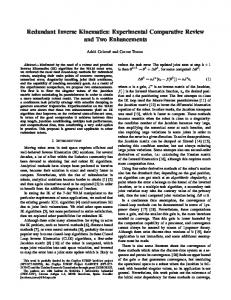
(17) To implement the inverse kinematics model, a spatial trajectory as shown in Fig. 3 is assumed. The spatial displacement components of the trajectory are based on biomechanics curves presented in [14] and [15]. The proposed method can be applied for any general case. It is possible to prescribe a trajectory describing a general curve in space, which means that the trajectory must not be necessarily in a straight line. The orientation of the center of mass and foot were taken as in Fig. 4. It describes the trajectory of the feet and center of mass during a complete gait cycle, described by 10 points. In this discrete gait cycle there are 9 different points of the center of mass trajectory, since the 5th and 6th pose are the same. Related to each

171

to obtain the general inverse kinnematics model of the leg, one has to take into account that the basee frame in the foot also describes a trajectory, since it is moving. The T transformation, which gives the spatial position and orientationn of the foot, is called ୤୭୭୲ . This fact complicates the inverse kinematics k considerably. It makes sense to represent the structture initially in a canonic form. Therefore, for an intermediatee simplification, the base frame is taken in the heel and this sepparates the transformation from the initial frame in the toes to thee heel. This transformation will be denoted ୆ . In addition, thee end effector frame is moved intermediately into the sphericaal joint. The complete model has to include therefore a transformatioon to change from the spherical joint frame to the center of mass fram me, which is the coordinate system in which acceleration and orientation o are measured. This transformation is denoted୉ . Thhe spatial position and orientation of the center of mass is denoted୫ୟୱୱ . Considering all the above transformations, the inverse kinnematics model is given by (19) and after some manipulation by (20)). Equation (20) separates the 6R structure into a left and a right constraint manifold. Since thee humanoid robot kinematic chain contains a spherical joint in thee hip, its inverse kinematics belongs to a special case as presented in [22]. Therefore, it is possible to represent the knee joint on the leeft side of the equation together with the ankle joints, and the spheriical joint in the right side. The left structure is a canonical structurre, and one can use the hyperplanes of the 3R canonical serial chainn in function of v2. The right side is the arbitrary spherical joint casee, in which the position of the base is represented by EE, given by (21).

Vertical Disp.[mm]

foot there are 5 points, since during the stancce period the position is constant. The trajectory of the heel is also reccorded, since the sensor for experimental verification was positioned in this point.

1-

2-

6-

7-

3-

4-

5-

89Figure 2. Poses during gait cycle. c

10-

150

Right Left CoM

100 50 0

0

0.2

0.4

0.6

0.8

1

1.2

1.4

Time [sec] Lateral Disp.[mm]

100 Right Left CoM

50 0 -50

0

0.2

0.4

0.6

0.8

1

1.2

1.4

Posterior Disp.[mm]

Time [sec] 100 Right Left CoM

50 0 -50 -100

0

0.2

0.4

0.6

0.8

1

1.2

TABLE II. DENAVIT-HARTENB BERG PARAMETERS OF THE 6R CHAIN. ݀௜ ߙ௜ ‫ݑ‬௜ ݅ ܽ௜ 1 0 0 0 ‫ݑ‬ଵ 2 0 0 ݈ଶ ‫ݑ‬ଶ 3 0 0 ݈ଷ ‫ݑ‬ଷ 4 0 0 െߨȀʹ ‫ݑ‬ସ 5 0 0 ߨȀʹ ‫ݑ‬ହ ൅ ߨȀʹ 6 0 0 0 ‫଺ݑ‬

1.4

Time [sec]

Figure 3. Displacement components of the cennter of mass and feet’s trajectory.

‫ܧܧ‬௙௢௢௧ Ǥ ܶ஻ Ǥ ‫ܯ‬ଵ Ǥ ‫ܩ‬ଵ Ǥ ‫ܯ‬ଶ Ǥ ‫ܩ‬ଶ Ǥ ‫ܯ‬ଷ Ǥ ‫ܩ‬ଷ Ǥ ‫ܯ‬ସ Ǥ ‫ܩ‬ସ Ǥ ‫ܯ‬ହ Ǥ ‫ܩ‬ହ Ǥ ‫ ଺ܯ‬Ǥ ‫ ଺ܩ‬Ǥ ܶா ൌ ‫ܧܧ‬௠௔௦௦ ି ‫ܯ‬ଵ Ǥ ‫ܩ‬ଵ Ǥ ‫ܯ‬ଶ Ǥ ‫ܩ‬ଶ Ǥ ‫ܯ‬ଷ Ǥ ‫ܩ‬ଷ ൌ ‫ܧܧ‬Ǥ ‫ି ଺ܩ‬ଵ Ǥ ‫ି ଺ܯ‬ଵ Ǥ ‫ܩ‬ହ ିଵ Ǥ ‫ܯ‬ହ ିଵ Ǥ ‫ܩ‬ସ ିଵ Ǥ ‫ܯ‬ସ ିଵ

with,

ିଵ ‫ܧ‬௙௢௢௧ Ǥ ‫ܧܧ‬௠௔௦௦ Ǥ ܶா ିଵ ‫ ܧܧ‬ൌ ܶ஻ ିଵ Ǥ ‫ܧܧ‬

(19) (20) (21)

Since the spherical joint is on the right side, represented by t be taken into account and in the inverse index -1, this fact has to equations of the hyperplanes thee values of the DH-parameters have to be transformed to reflect it. The following transformations are monstrated that the inverse matrix, in derived in [22]. There, it is dem this case the spherical joint sttructure, can be related to the old hyperplanes by changing the vallues as in (22). Figure 4. Proposed trajectory and orientation of the foot and center of mass (values in mm).

a3 = 0, d3  d4, al1  al5, al2  al4, al3 = 0 (22) Considering (20), it is poossible to obtain the polynomial expressions of the inverse kinem matics model of the humanoid robot as described in the following steeps:

IV. INVERSE KINEMATIICS In a first step the inverse kinematics moddel is derived taking the Denavit-Hartenberg parameters of a 6R strructure for each leg as presented in Tab. 2. In this case, the base frame is located in i the first joint of the structure and the end effector frame is in itss last joint. The pose of the end effector related to the base is then described by ܶଵ଺ ൌ ‫ܯ‬ଵ Ǥ ‫ܩ‬ଵ Ǥ ‫ܯ‬ଶ Ǥ ‫ܩ‬ଶ Ǥ ‫ܯ‬ଷ Ǥ ‫ܩ‬ଷ Ǥ ‫ܯ‬ସ Ǥ ‫ܩ‬ସ Ǥ ‫ܯ‬ହ Ǥ ‫ܩ‬ହ Ǥ ‫ ଺ܯ‬Ǥ ‫଺ܩ‬ (18) In (18) yields a 4x4 matrix expressed inn dual quaternion form, when taking the Study parameters as dissplacement parameters. These expressions represent the movement of o the 6R chain. In order

1- For each pose of the leg obbtain the matrices ‫ܧܧ‬௙௢௢௧ ǡ ‫ܧܧ‬௠௔௦௦ which represent the spatial poosition and orientation of foot and center of mass. 2- Substituting the Denavit-Harttenberg parameters the matrixes ܶ஻ and ܶா are computed, using (15)). 3- Obtain the kinematic mappingg of the matrices ܶ஻ ǡ ‫ܧܧ‬௙௢௢௧ ǡ ‫ܧܧ‬௠௔௦௦ and ܶா employing the Study paarameters from (10) and (11). The dual quaternion representation enables to obtain the inverse of

172

ܶ஻ ǡ ‫ܧܧ‬௙௢௢௧ and ܶா easily. Then (21) allows to compute the dual quaternion EE. 4- The left chain in (20) is a canonical 3R which can be represented by 4 hyperplanes in function of v2 and the D-H parameters of the structure. 5- The right chain represents a spherical joint which also can be represented by 4 hyperplanes. These 4 equations include the Denavit-Hartenberg parameters of the structure and the EE pose. 6- The value v2 of the second joint is obtained as intersection of eight hyperplanes (Hi) by computing the determinant, |h1(v2), h2(v2), h3(v2), h4(v2), h5, h6, h7, h8| , (23) where hi are the hyperplane coordinates of Hi, i = 1, . . . , 8. Zeroing the determinant yields a univariate polynomial P of degree four in v2, P1.v24 + P2.v23 + P3.v22 + P4.v2 +P5 = 0 (24) The solution of the (24) yields four values for v2, where P1, P2, P3, P4 and P5 are constants, which depend on the D-H parameters and the EE pose. The next steps are repeated for each of the four values of v2. 7- Replacing the v2 value in the hyperplane equations of steps 4 and 5, results in a system of 8 equations with the unknowns (x0,x1,x2,x3,y0,y1,y2,y3). The solution of this system gives the pose S in which the right and left chain coincide. A possible solution of this system is the point (0,0,0,0,0,0,0,0) which is not considered because it does not correspond to a valid pose of the robot. So, 7 hyperplane equations and the normalization condition represented by x0=1 are taken for computation of the unknowns; 8- The left chain also can be represented by four hyperplanes in function of v1. Taking one of these hyperplanes and the pose S, is possible to compute the value of v1; 9- The left chain also can be represented by four hyperplanes in function of v3. Taking one of these hyperplanes and the pose S, is possible to compute the value of v3; 10- At this step all joint values of the left chain are known. Therefore, it is possible to obtain the following (25) from (20). (25) ‫ܯ‬ସ Ǥ ‫ܩ‬ସ Ǥ ‫ܯ‬ହ Ǥ ‫ܩ‬ହ Ǥ ‫ ଺ܯ‬Ǥ ‫ ଺ܩ‬ൌ ܵ ିଵ Ǥ ‫ܧܧ‬ ିଵ In which ܵ is the inverse of pose S. This results in a system of 8 equations and 3 unknowns: v4, v5 and v6. It is possible to normalize both sides of the equations by the first equation. In addition, in this particular case it is observed that the last equation is 0=0. The remaining 6 equations are linearly dependent, namely the last 3 equations are 3 times the first three. Altogether this results in a system of 3 equations with 3 unknowns as follows:

E1=(v5*(v4 - v6))/(v4*v6 - 1); E2=- v5 - (2*v5)/(v4*v6 - 1); E3=-(v4 + v6)/(v4*v6 - 1);

For each of the 10 poses, the inverse kinematics model yields 8 possible solutions (Si) of the joints. It is possible to implement an algorithm to select one of the 8 solutions giving practical values applied to the humanoid robot. In this case, one of the asked conditions is to select solutions with u30, since the knee cannot bend in the opposite direction. The second condition is that all 6 angles are between +/-120 degrees, since during gait, in general, any joint does not move with amplitudes outside of this range. TABLE III. JOINT ANGLES OBTAINED AT 10 POSES (ANGLES IN DEGREES). u1 u2 u3 u4 u5 u6

P1

P2

P3

P4

P5

P6

P7

P8

P9

P10

0,00 38,76 -70,61 31,84 0,01 0,0

5,04 42,25 -74,55 32,29 -5,03 0,01

8,28 43,33 -76,45 33,12 -8,27 0,01

6,75 35,75 -74,60 38,83 -6,74 0,01

2,71 30,13 -70,12 39,98 -2,70 0,0

0,00 31,82 -70,60 38,78 0,01 0,0

-2,69 32,61 -69,37 36,76 2,70 0,01

-4,33 33,50 -68,40 34,89 4,34 0,01

-4,35 35,26 -69,17 33,90 4,36 0,01

-2,71 37,38 -70,62 33,23 2,72 0,0

V. NUMERICAL RESULTS

40

164.5 164

VerticalFoot [mm]

163.5

30 25 20

20

10 Pose

0

35

8

2

6

0

4 2 0 -2

20

10 Pose

0

0

10 Pose

20 0 -20

20

0

10 Pose

20

0

10 Pose

20

80

-2 -4 -6 -8

40

PosteriorFoot [mm]

165

60 PosteriorCoM [mm]

45 LateralCoM [mm]

166 165.5

LateralFoot [mm]

VerticalCoM [mm]

In this section the desired trajectory, based on human gait, is compared with the angles for the simulated trajectory obtained by inverse kinematics model. In order to simulate the trajectory the forward kinematics model is used as presented in Section 3. In Fig. 5 the points belong to the simulated poses and the lines connect the proposed poses. It is observed that simulated trajectory give the same poses as the proposed one.

0

10 Pose

60 40 20 0

20

Figure 5. Proposed and simulated trajectories.

The lines just connect the 10 first proposed poses, since it is assumed that the simulated gait repeats the same joint angles in each cycle, which can be seen in the sequence of points from pose 10 to 20. The proposed method can be applied for any general trajectory in space. In addition, it is possible to choose different orientations for the center of mass and foot. It is only necessary to ensure that the proposed pose is on the Study quadric and inside of the workspace of the leg. In Fig. 6, a curved trajectory is shown and Tab. 4 displays the corresponding values of the joints at the 10 poses.

(26)

In (26) E1, E2 and E3 are constants which are obtained by computing the S and EE entries for each value of v2. 11- Solving the system of (26) yields 2 values for v4, v5 and v6 each. The total of solutions comprises 4 values of v2, 4 values of v1 and v3 and 8 values of v4, v5 and v6. It is important to mention that with this algorithm all polynomial expressions for the inverse kinematics can be obtained in a symbolic form, which results in generic expressions for each joint. This algorithm was implemented in a Matlab routine in order to obtain the generic expressions and to

160 Right Left CoM

140 120 100 Lateral Disp.[mm]

analyze the results numerically. To verify the model the displacement and orientation of 10 poses, inspired by human gait were specified to calculate the joint angles. These 10 poses represent a complete gait cycle. The first 5 poses are related to the poses in which the foot is in movement, and the last 5 poses are related to the poses in which the foot is on the ground. The cycle gait is repeated for each leg. While one of the legs takes the joint angles of the first 5 poses, the other takes the joint angles of the last 5 poses. Tab. 3 displays the angle values obtained by the inverse kinematics model for the proposed trajectory.

80 60 40 20 0 -20 -20

0

20

40

60 80 Posterior Disp.[mm]

100

Figure 6. Curve trajectory.

173

120

140

TABLE IV. (DEGREES). u1 u2 u3 u4 u5 u6

P1 0,30 38,75 -70,61 31,85 -0,29 -5,00

JOINT

P2 5,04 42,25 -74,55 32,29 -5,03 0,00

P3 8,28 43,33 -76,45 33,12 -8,27 0,00

ANGLES P4 6,75 35,75 -74,60 38,83 -6,74 0,00

FOR

P5 3,13 30,39 -70,12 39,73 -3,11 5,00

P6 0,30 31,83 -70,60 38,77 -0,29 5,00

A CURVE P7 -2,69 32,61 -69,37 36,76 2,70 0,00

P8 -4,33 33,50 -68,40 34,89 4,34 0,00

[8]

TRAJECTORY P9 -4,35 35,26 -69,17 33,90 4,36 0,00

P10 -2,52 37,61 -70,62 33,00 2,53 -5,00

[9]

[10]

[11]

VI. CONCLUSION The proposed method gives a closed form algorithm to obtain the inverse kinematics of a humanoid robots which can be used to control systems and to simulate different spatial trajectories with human behavior. The polynomial equations used to represent the inverse kinematic model are an advantage for the control applications since it does not use trigonometric operations. Another advantage is the fact that the trajectory is defined by general spatial curves, for both center of mass and foot, independent of the division of robot gait in a frontal and lateral planes, which is proposed in different methods found in literature. A general spatial trajectory gives a humanoid robot gait a behavior more similar to the human gait, which is not observed in several applications. The proposed approach defines initially 10 poses of a desired trajectory. The whole trajectory can be found by using dual-quaternion interpolation, which is easier if compared with other methods. A contribution for future works is the fact that the kinematic analysis of mechanisms considering dual-quaternions is singularity free in the model and also when used to represent the signals from sensors. This is an important advantage of this approach. If the orientation of the system is measured considering Euler Angles, it can result in singularity of the data representation also in cases that the mechanism is not in a singular pose. This is called Gimbal-Lock problem and occurs if the sensor, for example, is positioned with an angle of 90 degrees around it pitch direction. Dual quaternion representation of the data avoids this problem. Since sensors give feedback to the inverse kinematics model by dual-quaternions, the movement can be directly obtained with the iterative algorithm proposed.

[12]

[13]

[14]

[15]

[16] [17]

[18]

[19]

[20]

[21]

ACKNOWLEDGMENT [22]

We thank the CNPq for sponsoring the project in “Science Without Borders” program and the Innsbruck members for the contribution in this work, all technical support, receptivity and partnership during this year of research and great learning.; The authors also are thankful to CAPES, UFU, FEMEC, FAPEMIG and EDROM for the partial financial support of this research.

[23] [24]

[25]

REFERENCES [1]

[2]

[3]

[4]

[5]

[6]

[7]

[26]

Kofinas N., Orfanoudakis E., Lagoudakis M.: Complete Analytical Inverse Kinematics for NAO, Proceedings of the 13th Int. Conf. on Auton.Robot Systems and Competitions, Portugal, pp. 1-6, 2013. Kofinas N.: Forward and Inverse Kinematics for the NAO Humanoid Robot, Diploma Thesis, Depart. of Electronic and Computer Engineering, Technical University of Crete, July 2012. Zorjan, M. and Hugel, V. “Generalized Humanoid Leg Inverse Kinematics to Deal With Singularities”, Proc. IEEE Int. Conf. on Robotics and Automation. 2013. Mistry, M.;Nakanishi, J.;Cheng, G.;Schaal, S.. Inverse kinematics with floating base and constraints for full body humanoid robot control, IEEE-RAS Inter. Conf. on Humanoid Robots. 2008. Zadeh, S.J.; Dept. of Comput. Eng., Shiraz Payame Noor Univ., Shiraz, Iran ; Khosravi, A. ; Moghimi, A. ; Roozmand, N. A review and analysis of the trajectory gait generation for humanoid robot using inverse kinematic. Electronics Computer Technology (ICECT), 2011. Ali, M. A., Park, H. A., Lee, C. S. G. Closed-Form Inverse Kinematic Joint Solution for Humanoid Robots. The 2010 IEEE/RSJ International Conf. on Intelligent Robots and Systems, Taipei, Taiwan. 2010. Meredith, M., Maddock, S. Real-Time Inverse Kinematics: The Return of the Jacobian. University of Sheffield, United Kingdom. 2015.

[27] [28] [29] [30] [31] [32]

[33]

[34]

174

Williams II, R.L.. Darwin-Op Humanoid Robot Kinematics. Proceedings of the ASME 2012 International Design Eng. Technical Conferences & Computers and Information in Eng. Conference. 2012. Rokbani, N., Alimi, A. M.. “IK-PSO, PSO Inverse Kinematics Solver with Application to Biped Gait Generation”. International Journal of Computer Applications (0975 – 8887) Volume 58– No.22. 2012. Nunez, J. V., Briseno, A., Rodriguez, D. A., Ibarra, J. M., Rodriguez, V. M.. Explicit analytic solution for inverse kinematics of Bioloid humanoid robot. DOI 10.1109/SBR-LARS.2012.62, 2012. Kenwright, Ben. “A Beginners Guide to Dual-Quaternions: What They Are, How They Work, and How to Use Them for 3D Character Hierarchies”, The 20th Intern. Conf. on Computer Graphics, Visualization and Computer Vision, WSCG 2012, pp.1-13. M. Schilling, “Universally manipulable body models — dual quaternion representations in layered and dynamic MMCs,” Autonomous Robots, 2011. Q. Ge, A. Varshney, J. P. Menon, and C. F. Chang, “Double quaternions for motion interpolation,” in Proceedings of the ASME Design Engineering Technical Conference, 1998. Wiebren Zijlstra; At L. Hof. Assessment of spatio-temporal gait parameters from trunk accelerations during human walking. Gait and Posture Journal. 2002. Li-Shan Chou; Kenton R. Kaufman ; Robert H. Brey ; Louis F. Draganich. Motion of the whole body’s center of mass when stepping over obstacles of different heights. Gait and Posture Journal. 2000. D. R. Walter and M. L. Husty. On Implicitization of Kinematic Constraint Equations. Machine Design & Research, 26:218–226, 2010. Husty, M. L., An Algorithm for Solving the Direct Kinematic of General Stewart-Gough Platforms, Mechanism and Machine Theory, vol. 31, No. 4, pp. 365-380, 1996. Husty, M. L., Karger, A., Self-Motions of Griffis-Duffy Type Platforms, Proceedings of IEEE conference on Robotics and Automation (ICRA 2000), San Francisco, 7–12, 2000. Husty, M. L., Karger, A., Self motions of Stewart-Gough platforms, an overview. Proceedings of the workshop on fundamental issues and future research directions for parallel mechanisms and manipulators, Quebec City, 131 – 141, 2002. Husty, M., Pfurner, M., Schröcker, H.-P., Brunnthaler, K.. Algebraic methods in mechanism analysis and synthesis. Robotica, 25(6):661675, 2007. Walter, D.R., Husty, M.L., Pfurner, M., A Complete Kinematic Analysis of the SNU 3- UPU Parallel Manipulator In: D.J. Bates, GM Besana, S. Di Rocco and C.W. Wampler, editors, Contemporary Mathematics, Vol. 496, American Mathematical Society, p. 331-346, 2009. ISBN: 978-0-8218-4746-6. Pfurner, M.. Analysis of spatial serial manipulators using kinematic mapping. PhD thesis, University of Innsbruck. 2006. Euler, L.. Formulae generales pro translatione quacunque corpum rigidorum. Novi Commentari Acad. Petropolitanae, 20:189–207, 1776. Kenwrigth, B. Inverse Kinematics with Dual-Quaternions, Exponential-Maps, and Joint Limits. International Journal on Advances in Intelligent Systems, vol 6 no 1 & 2. 2013. Bottema, O., Roth, B.. Theoretical Kinematics, volume 24 of NorthHolland Series in Applied Mathematics and Mechanics. North-Holland Publishing Company, Amsterdam, New York, Oxford, 1979. McCarthy, J.M.. Geometric Design of Linkages, volume 320 of Interd. Applied Mathematics. Springer-Verlag, New York, 2000. Cox, D., Little, J., O’Shea, D., Ideals, Varieties and Algorithms, 3rd. edition, Springer, 2007. J. M. Selig, Geometric Fundamentals of Robotics, Monographs in Computer Science, Springer, New York, 2005. G. H. Golub and C. F. Van Loan, Matrix Computations, Baltimore: Johns Hopkins University Press, third ed., 1996. E. Study, Geometrie der Dynamen, B. G. Teubner, Leipzig, 1903. E. Study, Von den Bewegungen und Umlegungen, Math. Ann., 39 (1891), pp. 441-566. 1891. Husty, M., Schröcker, H.-P.. Algebraic geometry and kinematics. In Ioannis Z. Emiris, Frank Sottile, and Thorsten Theobald, editors, Nonlinear Computational Geometry, volume 151 of The IMA Volumes in Mathematics and its Applications, chapter Algebraic Geometry and Kinematics, pages 85-107. Springer, 2010. J. Denavit and R.S. Hartenberg. A Kinematic Notation for Lower-Pair Mechanisms Based on Matrices. Journal of Applied Mechanics, 77:215–221, 1955. M.L. Husty, M. Pfurner, and H.-P. Schröcker. A new and efficient algorithm for the inverse kinematics of a general serial 6R manipulator. Mechanism and Machine theory, 2006.