Hybridizing Data Stream Mining And Technical Indicators In Automated Trading Systems Michael Mayo Department of Computer Science University of Waikato Hamilton, New Zealand
[email protected]
Abstract. Automated trading systems for financial markets can use data mining techniques for future price movement prediction. However, classifier accuracy is only one important component in such a system: the other is a decision procedure utilizing the prediction in order to be long, short or out of the market. In this paper, we investigate the use of technical indicators as a means of deciding when to trade in the direction of a classifier’s prediction. We compare this “hybrid” technical/data stream mining-based system with a naive system that always trades in the direction of predicted price movement. We are able to show via evaluations across five financial market datasets that our novel hybrid technique frequently outperforms the naive system. To strengthen our conclusions, we also include in our evaluation several “simple” trading strategies without any data mining component that provide a much stronger baseline for comparison than traditional buy-and-hold or sell-and-hold strategies.
1
Introduction
Analysing a financial market is a necessary precursor to the development of any trading strategy for that market. The type of analysis can vary greatly. For example, fundamental analysis is concerned with the broad economic factors and sweeping long term trends of a market [1]; technical analysis is concerned with finding clues to future price movements in historic market data and other variables [2]; and sentiment analysis involves gauging the opinion of market participants as to overall market direction [3]. Trading strategies may involve one, two or all of these methods of analysis. Our research falls squarely into the technical analysis camp. Over the past hundred years or so, numerous technical indicators and technical charting methods (such as trend lines) have been developed for so-called “price chart reading” (e.g. [4]). These indicators and methods are now so firmly entrenched in the psychology of market participants that they often become self-fulfilling prophecies rather than independent predictors. With the advent of computers, these traditional indicators are now considerably easier to compute, and literally every trader can have a hundred or so different indicators available at her fingertips.
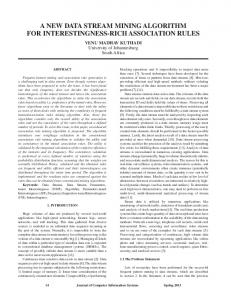
In terms of research, academics routinely apply new computerised methods such as data mining (e.g. [6], [8]), neural networks (e.g. [5], [7], and [10]), evolutionary algorithms (e.g. [9]), and recently data stream mining ([11]) to the markets in order to develop newer and better trading techniques, but also to better understand how the markets work. In this paper, we describe one such new technique which fuses the predictions made by a data mining classifier with a decision procedure based on technical analysis. The simple rule is that both types of analysis must agree before a trade in the predicted direction is made; if they disagree, no action is taken regardless of the classifier’s prediction. Our results show that in most cases, performance using this rule increases significantly compared to a trading system that only follows the classifier’s recommendations. Furthermore, the number of trades (and this applies even to the situations where there is no significant improvement in trading performance) is considerably reduced – to around 50% in many cases – leading therefore to much reduced transaction costs. We also provide a much more solid baseline for our experimental evaluations. Often in this field, it is considered “standard” to compare new strategies to buy-and-hold (whereby a long position is established at the beginning of the evaluation period and held to the end) or sell-and-hold (in which a short position is established and held to the end). The returns Fig. 1: Daily closing prices for the EURUSD marof the buy-and-hold or sell-and-hold ket, 23 May 2003 - 3 Dec 2010. strategies can then be compared to that of the new method under consideration. However, in modern markets, overly simplistic strategies such as buyand-hold frequently underperform as Figure 1 illustrates. This figure shows the daily closing prices for the EURUSD or “Eurodollar” market over the period from 23 May 2003 to 3 Dec 2010. The first closing price at the start of the period is $1.16 and the final closing price is $1.32 – representing a paltry 13.7% return (not annualized!) for a buy-andhold strategy over a nearly 7 year period. Despite this, an inspection of the price series shows that price swung Fig. 2: Daily closing prices for the AUDJPY forex greatly several times in amounts far market, 1 Dec 2003 - 3 Dec 2010. exceeding this net 13.7% movement. In fact, the highest recorded price is
around $1.60 and the lowest below $1.10. Clearly, any strategy just a little more intelligent than buy-and-hold could capture vastly more profit. Yet many papers compare their new “intelligent” strategy to buy-and-hold or sell-and-hold. A similar argument can be made for Figure 2, which shows prices for the Australian Dollar/Japanese Yen (AUDJPY) market. We advocate significantly more challenging baseline strategies inspired by (and including) the simple strategies first proposed by Tiˇ no [12], which are designed specifically to be conducive for statistical significance testing. In the next section, we outline our new method in more detail, discussing the technical and classifier components of the system as well as the strategy execution on a price series. In Section 3 we detail the experimental setup, in particular focussing on the baseline simple strategies (superior to buy-and-hold) that were used for comparison, as well as the evaluation measures usede. Section 4 describes the actual evaluation itself, with the datasets, and then the results. Finally, Section 5 concludes the paper.
2
Proposed New Trading Strategy Framework
Our hybrid framework for trading strategy design consists of two main components: a technical component based on standard technical indicators, and a data stream mining component, which is an abstaining classifier trained on a stream of historic price data. Besides price, the values of various indicators and other indexes may also be included in the stream. 2.1
The Technical Trading Rule (or Filtering) Component
A technical trading rule generally involves the computation of one or more technical indicators from historic price data. Because technical indicators are often designed to gauge a market’s price trend direction, a trading rule is essentially a filter for trading actions, for example to rule out buy trades when the market is trending down. One of the simplest technical indicators is the Simple Moving Average (SMA) [4]. Two instances of this indicator are depicted in Figure 3 where they are overlaid on the closing price series for the USDJPY market from the period 15 May 2003 to 3 Dec 2010. The dark, slower-moving line is the 200-period SMA while the medium-grey, faster-moving line is the 20-period SMA. Because the 200-period SMA lags behind the 20-period SMA, a good technical trading rule (and the one adopted in this paper) is to go long (buy) only if the 20 SMA is above the 200 SMA; and to go short (sell) only if the 20 SMA is below the 200 SMA. We can see that using this rule would have resulted in mostly buying in the approximate period May ’05 to May ’07 because the 20 SMA is mostly above the 200 SMA during this period. Thereafter, the 20 SMA is mostly below the 200 SMA and therefore most trades would have been short (selling).
Fig. 3: Daily closing prices for the USDJPY forex market, 15 May 2003 - 3 Dec 2010, with the 20 and 200 period SMAs overlaid.
Note that the direction of the technical trading rules does not force a trade to be made; rather it is applied as a filter to eliminate potentially incorrect predictions made by the abstaining classifier component described next. 2.2
The Abstaining-Classifier Component
The abstaining-classifier component is a machine learning classifier capable of abstaining from a prediction if the uncertainty is too high. The simplest way to achieve this is to have the classifier predict not a binary direction (e.g. up or down) for the market over the next period, but a probability distribution over market directions. If the probabilities are within a small deviation of 0.5 (which in our case is 0.0001), then the classifier abstains from making a prediction and there is no trade. 2.3
Strategy Execution
The basic rule is that in order for a trade to occur, the most likely market direction (up or down) as predicted by the classifier must agree with the technical trading trade. In other words, the 20-period SMA must exceed the 200-period SMA and the classifier must predict an upwards price movement in order for a long trade to happen; vice-versa for a short trade. If the classifier abstains or the classifier’s prediction conflicts with the technical trading rule, then no trade is made. We also use a standard “sliding window” method for executing our strategy. The basic idea is that (as opposed to performing a single train/test split for an entire dataset), a new classifier is instead trained for every single prediction that needs to be made. The training data for the classifier is obtained by sliding a 200-day fixed-size window along the price stream, so that only the most recent data (up to and excluding the test instance) is used for prediction. Using this
method, older data is gradually discarded. Each instance in our data stream consists of 10 price points leading up to the day to be predicted. Also, it should be noted that instead of raw prices, we use the log-return values: rn = sgn(cn − on ) × log(K|cn − on |)
(1)
where rn is the log return, on is the opening price of the nth day, cn is the same day’s closing price, sgn(.) is the sign function, and K is an abitrary constant. This feature proved far superior to raw price during initial testing. The strategy assumes that trades are held only during market opening hours, and that they can only be initiated at the market open (i.e.. a buy at price on ), and closed at the end of the day (at price cn ). No positions are allowed to be held overnight or over weekends, which eliminates the effects of gap ups and gap downs. No stops are used, which means that we do not need to be concerned with the order that prices were visited during the day – only on and cn are significant. Finally, the decision to trade and the direction of the trade for the next day are made at the immediate close of the current day, as soon as the SMAs and the classifier can be updated.
3
Methodology
In this section, we present four different experimental conditions that we were concerned with, and briefly describe the trading strategy evaluation measures used. 3.1
The Four Experimental Conditions
Simple, Non-Filtered In the simple, non-filtered case, we adopt Tiˇ no’s [12] four proposed baseline strategies. They are SimpleL , a strategy that goes long every day; SimpleS , a strategy that goes short every day; SimpleT R , a trend following strategy that buys if the previous day’s close was higher than its open, and sells whenever yesterday’s close was below its open; and SimpleCT , a countertrend strategy that does the opposite of SimpleT R . Note that while SimpleL and SimpleS are superficially similar to buy-andhold and sell-and-hold, they exit the market at the close of each day, and re-enter the next day. Buy-and-hold and sell-and-hold on the other hand enter the market once at the period beginning and exit once at the end. Simple, Filtered The simple, filtered strategies are four additional strategies that are introduced in this paper. The basic idea is to take Tiˇ no’s four baseline strategies described above and apply the technical trading rule described in Section 2.1. This generates four new strategies which are filtered – that is, they are only in the market if the trade direction agrees with the technical trading rule, and they are out of the market (flat) otherwise.
Machine Learning, Non-Filtered In the Machine Learning (ML) non-filtered set of strategies, we use an abstaining classifier to predict market direction and trade whenever the classifier makes a prediction. The classifiers we use are Naive Bayes (NB) [13], Support Vector Machines (SVMs) [15] and Random Forest (RF) [16]. We also add a simple classifier, ZeroR (0R) which only ever predicts the majority class from the 200-day training dataset. This serves as an additional baseline for the classifiers. The implementations of the classifiers are those found in Weka 3.6.6 [17] with all default parameters, bar the Random Forest classifier which consists of 100 instead of 10 random trees. Machine Learning, Filtered Finally, the set of strategies in this group represent our target group: they are a full implementation of the system described in Section 2 in which an abstaining classifier’s predictions are combined with a technical trading rule. They vary only in the choice of classifier. 3.2
Evaluation Measures
In this section, we briefly outline the evaluation measures we used. Accuracy The accuracy measures we report give the percentage of times that the strategy correctly predicts the market direction (up or down). We exclude situations where there is no trade (for example, because the classifier disagrees with the technical rule). Net Profit Ratio Most trading strategies are concerned with maximising net profit whilst minimising risk. This corresponds to having winning trades that return as much profit as possible, and losing trades that make minimal losses. One way to measure this is the Net Profit Ratio (NPR), in which total Net Profit (NP, i.e. sum of all wins from all winning trades less sum of losses from all losing trades) divided by Maximum Drawdown (MDD): NP (2) M DD In this ratio, the MDD is defined as the maximum drop in NP that a trading strategy experiences over a particular period. For example, if a strategy starts at $0 NP, then reaches $100 NP after some wins, then drops to $50 NP after some losses, and finally ends the testing period (after further wins and losses) with $120 net profit, then the MDD is $50 which corresponds to the largest drop of profits from $100 to $50. The NPR therefore would be $120 $50 = 2.4. Ideally, we want to find trading strategies with NPRs as high as possible. This will tell us that the strategy has a high NP relative to its MDD. Strategies that have a NPR of 1.0 or less are undesirable for actual live trading, because such a low NPR implies that the MDD is greater than (or at least equal to) the NP, which may make the strategy a riskier proposition. NPR =
Statistical Significance We also assess each trading strategy’s performance statistically using Monte Carlo Permutation Testing (MCPT) [18] [19]. MCPT takes the daily positions (long, short or flat) made by a strategy, and randomly permutes them M times to produce M randomized trading strategies or “samples”. It then computes the total NP of each sample and compares these using a conservative right-tailed test to the total NP achieved by the strategy. MCPT is useful for evaluating the statistical significance of a trading strategy because it makes no assumptions about the performances of other possible trading strategies – i.e. NPs achieved by the random strategies need not have a normal distribution, nor do they need to have a zero mean (which is a highly unlikely assumption in a strongly bullish or bearish market). Significance is reported for each Fig. 4: Daily closing prices for the GOOGLE stock market, 25 Oct 2004 - 3 Dec 2010. strategy as a p value, where a smaller p value indicates greater significance. Values less than 0.05 are significant at 95% confidence.
4
Evaluation
We now describe the evaluation and our results in detail. 4.1
Datasets
We acquired five daily streaming datasets from Dukascopy [20]. They are the EURUSD, AUDJPY and USDJPY datasets already discussed and depicted in Figures 1-3, along 5: Daily closing prices for the BOEING stock with two stock market datasets, one Fig. market, 17 Mar 2003 - 3 Dec 2010. for Google (Figure 4) and the other for Boeing (Figure 5). The data sets each comprise open, close, minimum and maximum prices for each trading day. We further added the 20 and 200 SMAs to the streams. In all cases, there are 2000 days worth of data, except for AUDJPY which has only 1832 days, and Google, which has 1583 days. EURUSD and USDJPY were chosen because they are the most commonly traded forex markets; AUDJPY was chosen because it is an interesting market with a high volume of carry trades;
and Google and Boeing were selected because they represent two different but popular companies in the stock market. In each dataset, predictions were not made for the first 210 days because these days were the minimum needed to construct a full dataset for training the classifiers given the window size of 200 and the instance size of 10. 4.2
Results
We executed each of the strategies in each of the four conditions (Filtered vs. non-filtered, simple vs. ML-based) on each of the five datasets. This gave a total of 16 × 5 = 80 experiments that were performed. To evaluate the effect of the classifier abstentions and technical filtering, we first of all counted the number of trades that were actually executed. They are given in Table 1. A key point from this table is that the effect of filtering varies massively. In some cases, the number of trades is reduced only somewhat, for example from 1790 to 1360 in the case of filtered 0R applied to EURUSD. However, in other cases the trade reduction is huge, such as the drop from 1790 trades to 476 trades in the case of Boeing with filtered SimpleL . This corresponds to trading about once every three or four days instead of every day. Strategy EURUSD USDJPY AUDJPY GOOGLE BOEING NON-SimpleL 1790 1790 1622 1373 1790 NON-SimpleS 1790 1790 1622 1373 1790 NON-SimpleT R 1790 1790 1622 1373 1790 NON-SimpleCT 1790 1790 1622 1373 1790 NON-0R 1716 1694 1597 1318 1689 NON-NB 1790 1790 1622 1373 1789 NON-SVM 1790 1790 1622 1373 1790 NON-RF 1750 1749 1597 1336 1736 FIL-SimpleL 1121 794 1097 910 1314 FIL-SimpleS 669 996 525 463 476 FIL-SimpleT R 924 896 850 742 904 FIL-SimpleCT 866 894 772 631 886 FIL-0R 1360 957 1152 896 1207 FIL-NB 1019 925 937 807 987 FIL-SVM 977 917 977 890 984 FIL-RF 971 918 909 794 934 Table 1: Number of trades by condition (row) and dataset (column).
Table 2 gives the overall accuracies. In most cases the accuracy is around 50%, with the exception of AUDJPY in which filtered SimpleL achieves about 55%. This can be most likely explained as long-bias due to the carry trade. The near-random degree of accuracy concurs with previous results such as [21] and [8] where only small gains in accuracy (about 1-2%) above random were achievable when new methods were tested. The NPRs for each strategy and each dataset are given in Table 3, which shows considerable variation. About half of the strategies fail to make any profit at all, ending the testing period with a net loss (negative NPR). Of those remaining, many have a NPR below 1.0, which suggests that these strategies tend to make large losses in comparison to their final net profit.
Strategy EURUSD USDJPY AUDJPY GOOGLE BOEING NON-SimpleL 49.4% 50.6% 55.1% 47.9% 49.5% NON-SimpleS 48.9% 48.7% 43.8% 47.6% 48.6% NON-SimpleT R 46.4% 46.8% 49.7% 48.0% 45.8% NON-SimpleCT 51.9% 52.5% 49.2% 47.5% 52.3% NON-0R 49.2% 51.1% 54.5% 47.4% 48.2% NON-NB 49.7% 50.6% 52.0% 47.3% 48.6% NON-SVM 50.6% 51.7% 51.7% 48.4% 49.1% NON-RF 48.9% 49.8% 51.8% 47.2% 49.8% FIL-SimpleL 50.6% 50.0% 55.2% 51.3% 50.0% FIL-SimpleS 51.4% 48.3% 44.2% 49.2% 50.2% FIL-SimpleT R 48.2% 46.2% 51.9% 49.3% 46.7% FIL-SimpleCT 53.8% 51.9% 51.4% 52.1% 53.5% FIL-0R 50.3% 50.1% 54.5% 49.3% 48.6% FIL-NB 51.0% 49.9% 53.6% 49.3% 49.2% FIL-SVM 51.7% 51.0% 53.2% 50.0% 50.0% FIL-RF 50.3% 49.7% 53.7% 48.7% 50.9% Table 2: Strategy directional accuracy by condition (row) and dataset (column).
On the other hand, there are a few strategies that are big winners in NPR terms. For example, the filtered SimpleCT strategy on EURUSD achieves a NPR of 2.142 – implying that more than $2 profit were made for each $1 of loss. However, this strategy does not include a classifier, and the strategies that did tended to perform not as well on the EURUSD Fig. 6: Daily equity curve for the Filtered SimpleCT strategy on EURUSD. The axes are day dataset. (x ) vs. profit (y, in points, 1 point=0.0001 dollars). The opposite is true however for the AUDJPY and BOEING datasets. In these experiments, filtered classifierbased strategies achieve NPRs of 1.444 and 3.909 respectively, with the classifiers being Naive Bayes in the first case and Random Forest in the second case. These two cases represent markets on which our new approach works exceedingly well. Strategy EURUSD USDJPY AUDJPY GOOGLE BOEING NON-SimpleL -0.058 -0.595 0.004 0.522 0.184 NON-SimpleS 0.068 1.280 -0.008 -0.571 -0.228 NON-SimpleT R -0.706 -0.755 -0.235 0.394 -0.436 NON-SimpleCT 1.487 2.485 0.506 -0.218 0.746 NON-0R 0.397 -0.818 -0.390 -0.661 -0.401 NON-NB 0.918 0.041 1.186 -0.853 -0.372 NON-SVM 1.408 1.204 0.400 -0.697 -0.261 NON-RF -0.448 -0.128 -0.029 -0.853 1.889 FIL-SimpleL 0.670 -0.917 -0.052 1.243 2.043 FIL-SimpleS 0.794 -0.267 -0.067 0.305 1.084 FIL-SimpleT R -0.299 -0.887 -0.280 1.475 0.560 FIL-SimpleCT 2.142 0.382 0.344 0.830 1.961 FIL-0R 0.871 -0.864 -0.361 -0.008 0.668 FIL-NB 1.229 -0.769 1.444 -0.535 0.585 FIL-SVM 1.362 -0.269 0.238 -0.157 1.012 FIL-RF 0.144 -0.598 0.044 -0.409 3.909 Table 3: Strategy net profit ratio by condition (row) and dataset (column).
Table 4 gives the statistical significance values. In this table, a lower value indicates greater significance. Comparing the two tables, we see that in many
cases, a low p value correlates to a high NPR. Note that there are only a handful of strategies that are significant at 95% level: they are non-filtered SimpleCT and SVM strategies applied to the USDJPY market (the SVM strategy has greater significance); and the Random Forest-based strategies applied to BOEING. Some of the other high-NPR also have low p values, but they are not quite significant, such as the non-filtered Naive Bayes strategy with a p value of 0.102 which is nearly significant at a level of 90%. Strategy EURUSD USDJPY AUDJPY GOOGLE BOEING NON-SimpleL 1.000 1.000 1.000 1.000 1.000 NON-SimpleS 1.000 1.000 1.000 1.000 1.000 NON-SimpleT R 0.868 0.976 0.701 0.378 0.781 NON-SimpleCT 0.132 0.025 0.300 0.622 0.220 NON-0R 0.369 0.903 0.808 0.864 0.666 NON-NB 0.238 0.480 0.102 0.978 0.739 NON-SVM 0.138 0.018 0.352 0.978 0.626 NON-RF 0.719 0.560 0.504 0.966 0.060 FIL-SimpleL 0.209 0.916 0.526 0.201 0.060 FIL-SimpleS 0.209 0.916 0.526 0.201 0.060 FIL-SimpleT R 0.593 0.991 0.665 0.229 0.326 FIL-SimpleCT 0.085 0.339 0.367 0.347 0.056 FIL-0R 0.249 0.974 0.680 0.530 0.328 FIL-NB 0.158 0.820 0.205 0.788 0.296 FIL-SVM 0.103 0.625 0.410 0.611 0.231 FIL-RF 0.455 0.779 0.511 0.703 0.017 Table 4: Strategy statistical significance by condition (row) and dataset (column).
The equity curves of some of the better-performing strategies are presented next. Figure 6 shows the reasonably good performance of the filtered simple countertrend strategy on the EURUSD market. Note that the strategy actually loses money for the first year or so before profits start to increase. Figure 7 shows the equity curves for the two highly-performing strategies applied to the USDJPY mar- Fig. 7: Daily equity curve for the Non-filtered CT (black line, upper) and SVM (grey line, ket, specifically the non-filtered coun- Simple lower) strategies on USDJPY. The axes are day tertrend strategy and the non-filtered (x ) vs. profit (y, in points, 1 point=0.01 Yen). SVM strategy. Although the latter strategy has a higher statistical significance according to permutation testing, the former strategy actually produces a greater NPR over time. This emphasizes one of the key points of the permutation test for trading strategies, which is that the test does not rank strategies according to profitability: instead, it ranks them according to how unlikely it would be for a random strategy to produce the same result. Figures 8 and 9 show further equity curves, this time for two filtered strategies, specifically Naive Bayes on AUDJPY and Random Forest on BOEING. Note than in all cases, the equity curves show the points or cents won. This
measurement is independent of position or account size. If the curves were depicted with account size on the y axis instead and compounding of position sizes was employed, it would be expected that the curves would be much steeper.
5
Conclusion
To conclude, we have demonstrated that a novel hybridized data mining/technical trading rule strategy can perform effectively and significantly in some markets. However, there is no single optimal or “holy grail” strategy that fits all five of our test datasets. Rather, each market appears to have its own dynamics and character, and therefore requires its own unique investigation. It is also known that markets change gradually Fig. 8: Daily equity curve for the Filtered Naive Bayes strategy on AUDJPY. The axes are day (x ) over time (i.e. the distribution of price vs. profit (y, in points, 1 point=0.01 Yen). changes is non-stationary), so the process of optimizing the hybrid strategy is likely to be continuous rather than a one-off event. We have also compared our “intelligent” strategies to a set of very strong simplistic strategies which can sometimes themselves yield high profits and nearstatistical significance. In this respect, our research here differs considerably from that of prior literature where the baseline strategy, if one is proposed, is most often an easily out-performed buy-and-hold strategy. We feel the more rigorous evaluations performed here give a more realistic view of the performance of our approach. There is also one caveat that should be made concerning this research: we have not included transaction and slippage costs in our simulations. For the forex markets, the transaction costs are very low compared to the stock market, but costs are changing rapidly with time. Slippage and costs are difficult to model because they are dependent on the broker as well as market conditions not available in the Fig. 9: Daily equity curve for the Filtered Random price data stream. Individuals conForests strategy on BOEING. The axes are day structing a live implementation of an (x ) vs. profit (y, in cents). automated trading system such as the one introduced here should make appropriate assumptions about their own costs when they evaluate potential strategies.
References 1. 2. 3. 4. 5.
Schwager, J. Futures: Fundamental Analysis Wiley (1995) Pring, M. Market Momentum McGraw-Hill Companies (1997) Saettele, J. Sentiment in the Forex Market Wiley (2008) Pring M. Technical Analysis Explained McGraw-Hill (2002) Y. Lean,K. Lai. Foreign Exchange Rate Forecasting with Artificial Neural Networks. Springer-Verlag, 2007. 6. Z. Liu, D. Xiu. “An automated trading system with multi-indicator fusion based on D-S evidence theory in forex market,” in Proc. Sixth International Conference on Fuzzy Systems and Knowledge Discovery, IEEE, 2009, pp. 239-243. 7. H. Ni, H. Yin. “Exchange rate prediction using hybrid neural networks and trading indicators,” Neurocomputing72:2815-2832, 2009. 8. R. Barbosa, O. Belo. “Autonomous Forex Trading Agents,” in Proc. 2008 International Conference on Data Mining, ICDM 2008, P. Perner Ed., LNAI 5077, pp. 389-403, 2008. 9. A. Hirabayashi, C. Aranha, H. Iba. “Optimization of the Trading Rule in Foreign Exchange using Genetic Algorithm,” in Proc. GECCO’09, pp. 1529-1536. 10. S. Walczak. “An Empiracal Analysis of Data Requirements for Financial Forecasting with Neural Networks” Journal of Management Information Systems 17(4), pp. 203-222. 2001. 11. Montana, G., Trianafyllopoulos, K., Tsagaris, T. Data stream mining for marketneutral algorithmic trading. Proc. Symposium on Applied Computing (SAC’08), 2008, pp. 966-970. 12. Tiˇ no, P., Schittenkopf C and Dorffner G. “Financial Volatility Trading using Recurrent Neural Networks.” IEEE Trans. on Neural Networks 12(4), pp. 865-874, 2002. 13. G John, P Langley. “Estimating Continuous Distributions in Bayesian Classifiers,” in Eleventh Conference on Uncertainty in Artificial Intelligence, San Mateo, 1995, pp. 338-345. 14. S. le Cessie, J.C. van Houwelingen. “Ridge estimators in logistic regression,” Applied Statistics 41(1): 191-201. 15. J. C. Platt, “Fast training of support vector machines using sequential minimal optimization,” in Advances in Kernel Methods – Support Vector Learning, B. Sch¨ olkopf, C. Burges, and A. Smola, Eds. MIT Press, 1998. 16. L. Breiman. “Random Forests”. Machine Learning 45(1):5-32. 17. M. Hall, E. Frank, G. Holmes, B. Pfahringer, P. Reutemann, and I. H. Witten, “The WEKA data mining software: An update,” SIGKDD Explorations, vol. 11, no. 1, 2009. 18. Aronson, D. Evidence-Based Technical Analysis: Applying the Scientific Method and Statistical Inference to Trading Signals. 19. Masters, T, Monte-Carlo Evaluation of Trading Systems. 2006. Available online at www.evidencebasedta.com/MonteDoc12.15.06.pdf, retrieved 13 Dec 2010. 20. Dukascopy Swiss Forex Bank & Marketplace, www.dukascopy.com. Data retrieved 4 Dec 2010. 21. “Evaluating the performance of adapting trading strategies with different memory lengths,” in Proc. Int. Data Eng. & Automated Learning (IDEAL 2009) Lecture Notes in Computer Science, 2009, Volume 5788/2009, pp. 711-718