1
Hyperbolic splines and nonlinear distortion Richard Martin, Ken Lever and Jeff McCarthy Abstract— Using M¨ obius transformations we consider how to interpolate a set of monotone increasing data points (xk , yk ) so that the interpolant is a smooth invertible function and that the interpolant and its inverse have the same simple functional form. We use our method to cancel jammerinduced distortion in a nonlinear channel. Keywords— Splines, invertibility, nonlinear distortion
I. Statement of the problem A set of data points D is given as D = {(x0 , y0 ), (x1 , y1 ), . . . , (xn , yn )}, obtained by ‘observing’ the function y = f (x) at certain places. Suppose that f is continuous and has a continuous inverse; without loss of generality, f is strictly increasing and x0 < x1 < · · · < xn , y0 < y1 < · · · < yn . It is desired to find a function fˆD : [x0 , xn ] → [y0 , yn ] that approximates f and interpolates these points. Furthermore fˆD must have the following properties: (P1) fˆD has continuous first (and possibly higher) derivative(s) (P2) fˆD is invertible1 and fˆD−1 = (fˆD )−1 . By D−1 , we mean the ‘inverse’ set of data points D−1 = {(y0 , x0 ), (y1 , x1 ), . . . , (yn , xn )}. It is important to appreciate the full implication of P2. The statement means that the functional approximation obtained by reflecting the data points in the line y = x and then interpolating them is precisely the inverse of the functional approximation obtained by interpolating the original data. The reason for condition P2 is that we may wish to model a nonlinear distortion with the view to correcting it; in that case the approximation must be invertible and the inverse should be easy to calculate. By requiring that fˆD−1 = (fˆD )−1 we ensure that the same model for the nonlinearity is obtained regardless of which of x and y is taken as the independent variable. Hence P2 asks for more than monotonicity. The ‘usual’ interpolative techniques do not obey P2. With polynomials, for example, fˆD and fˆD−1 would both be polynomials and so fˆD ◦ fˆD−1 could not be the identity mapping, and P2 would not be obeyed. The same objection applies to quadratic and cubic splines (see e.g. [1]) and to radial basis functions (see e.g. [2]). There is a simple interpolative technique that satisfies P2: the piecewise linear fit. Although this does not satisfy Published in IEEE Trans. Sig. Proc. 48, 6, 1825–28 (2000). E-mail:
[email protected] 1 i.e. there exists an inverse function f −1 such that f −1 (f (x)) = x for x ∈ [x0 , xn ].
P1, it is a step in the right direction, because piecewise linear functions do form a group under composition. The question is how to admit a larger class of functions to deal with curvature while preserving the group property. We argue that splines of the form x 7→ ax+b cx+d are an elegant and simple solution to this problem. Splines of the form linear linear fall into the class of rational splines, for which there has been an extensive amount of work in the last twenty years. Most of this work has been aimed at finding interpolatory functions which are ‘visually appealing’ (follow the trend of the data without additional inflections) or ‘shape-preserving’ (e.g. monotonicity, convexity, or positivity). While some work has been based on more traditional splines using extra information (e.g. [3], [4]), most has involved rational functions, including cubic cubic cubic cubic C 2 splines [5], quadratic C 2 splines [6] and linear C 2 splines [7]. Others have investigated parametric shape-preserving curves, using for example piecewise cubic [8] and cubic cubic [9]. In many of the above references (and others cited within them), ‘tension parameters’ are introduced, which in the limit lead to straight-line segments between points. It is an appropriate choice of these parameters which provides the shape-preserving property. While the curves to be described here will only be C 1 , as opposed to C 2 in several of the above references, we once again emphasise that the novelty of the approach described here is invertibility. ¨ bius functions and spline fitting II. Mo A. Group-theoretic properties It is an elementary fact that there is a close connection between transformations of the form x 7→ ax+b cx+d and twoby-two matrices. Specifically we may associate ( ) { [ ] } ax + b a b x 7→ ←→ k :k ∈R\0 . c d cx + d The reason why this association is important is that the composite of two M¨obius transformations corresponds to the product of their respective matrices. In particular, the inverse of the transformation x 7→ ax+b cx+d is given by x 7→ dx−b −cx+a , provided that the determinant ad − bc ̸= 0. Algebraically speaking we have exhibited a group isomorphism between the M¨obius functions and2 the group PGL2 (R). It is clear from the above remarks that piecewise M¨obius functions with continuous first derivative—we shall henceforth call them hyperbolic splines—form a group under 2 PGL (R) is the group under multiplication of real 2-by-2 matrices 2 modulo the equivalence relation of one matrix being a scalar multiple of the other.
2
composition. They will form the basis of the interpolation technique that we are going to use. B. Explicit construction The cornerstone of the interpolation technique is the following result. Lemma 1: For real numbers xk < xk+1 and yk < yk+1 , k+1 −yk write δk = xyk+1 obius function gk associated −xk . The M¨ with the matrix [ ][ ][ ] yk+1 − yk yk λk 0 1 −xk (1) 0 1 λk − 1 1 0 xk+1 − xk obeys gk (xk ) = yk , gk (xk+1 ) = yk+1 and gk′ (xk ) = λk δk ; it is unique in this respect. Further, gk′ (xk+1 ) = δk /λk , and if λk > 0 then gk is monotonic on [xk , xk+1 ]. Finally, gk−1 is given by [ ] [ −1 ][ ] xk+1 − xk xk λk 0 1 −yk . (2) 0 1 0 yk+1 − yk λ−1 k −1 1 The proof is straightforward. The middle matrix in (1) corresponds to a map fixing 0 and 1 and having derivative λk at 0; as is easily verified, no other M¨obius transformation has these properties. The outer two maps in (1) are responsible for mapping [xk , xk+1 ] to [0, 1] and [0, 1] to [yk , yk+1 ]; both are linear. Eq. (2) follows directly. The application of the Lemma is as follows. The form of the approximant fˆ : [x0 , xn ] → [y0 , yn ] is that in each subinterval [xk , xk+1 ] fˆ is a M¨obius function given by (1). As yet we have not defined the (λk ). The Lemma shows that regardless of the (λk ) the function fˆ must be continuous, so we just have to match the first derivative at the ends of the subintervals. The Lemma also tells us how to do this. Starting with λ0 which for the moment will be arbitrary we choose λ1 so that the pieces on [x0 , x1 ] and [x1 , x2 ] have equal first derivative at x1 . This requires λ1 = δ0 /(δ1 λ0 ). Continuing in this way we obtain the rest of the (λk ) by the recursion λk+1 = δk /(δk+1 λk ).
(3)
With this, the implementation could hardly be easier. In many applications, particularly those in which nonlinear distortion is being considered, the distortion function f is odd. In that case f (0) = 0 and we may assume that the data set D is {(0, 0), (x1 , y1 ), . . . , (xn , yn )}. We now discuss how to find λ0 . There are some situations in which the derivative is known at the left-hand end of D (or, as we discussed in the previous paragraph, at x = 0). In that case λ0 can be inferred from the derivative there. In other instances, particularly those in which f is odd, it could be reasonable to assume that f is almost perfectly linear near the origin, and that it would be valid to make fˆ linear in the first segment [0, x1 ]; that would be arranged by choosing λ0 = 1. Alternatively one might wish to approximate a known function f , as in Example 3 below, in which case λ0 can be adjusted by hand. Here is a method that works in the absence of such information. It is apparent that different choices for λ0 will produce interpolants of different twistiness (see Figure 1). Perhaps
therefore we should select λ0 so as to make the interpolant as ‘gentle’ as possible. To do this we define a function on fˆ that measures the curvature: ( ) Γ : fˆD 7→ max max(λk , λ−1 ) . (4) k 0≤k