I-Quest: An Intelligent Query Structuring Based on ...

Multimedia Tools and Applications, June 2009, Volume 43, Issue 2, pp 145-178. The final publication is available at at Springer via http://link.springer.com/article/10.1007/s11042-009-0262-3.

I-Quest: An Intelligent Query Structuring Based on User Browsing Feedback for Semantic Retrieval of Video Data Tarun Yadav ∗and Ramazan Sava¸s Ayg¨ un

†

Abstract In spite of significant improvements in video data retrieval, a system has not yet been developed that can adequately respond to a user’s query. Typically, the user has to refine the query many times and view query results until eventually the expected videos are retrieved from the database. The complexity of video data and questionable query structuring by the user aggravates the retrieval process. Most previous research in this area has focused on retrieval based on low-level features. Managing imprecise queries using semantic (high-level) content is no easier than queries based on low-level features due to the absence of a proper continuous distance function. We provide a method to help users search for clips and videos of interest in video databases. The video clips are classified as interesting and uninteresting based on user browsing. The attribute values of clips are classified by commonality, presence, and frequency within each of the two groups to be used in computing the relevance of each clip to the user’s query. In this paper, we provide an intelligent query structuring system, called I-Quest, to rank clips based on user browsing feedback, where a template generation from the set of interesting and uninteresting sets is impossible or yields poor results.

Keywords: Multimedia information retrieval, Semantic Retrieval, Relevance Feedback, User Browsing

∗ T. Yadav is with Broadband Enterprises. He was with Computer Science Department, Technology Hall N360, University of Alabama in Huntsville, Huntsville, AL 35899. Email: [email protected]. † R. Ayg¨ un is with Computer Science Department, Technology Hall N360, University of Alabama in Huntsville, Huntsville, AL 35899. Phone: 256-824-6455, Fax: 256-824-6239, Email: [email protected]

1

1

Introduction

There has been tremendous demand for on-line digital video in the last decade. This demand has been growing significantly since the beginning of this millennium. With the introduction of the MPEG-7 standard [1, 2], semantic video information can be stored and used to filter and manage multimedia content. However, the video retrieval process may be lengthy because of the naivete of the user and video data complexity. Especially for large multimedia collections, methods and tools need to be developed to help users retrieve videos. The complex structure of video data makes it difficult to structure accurate queries. There might be differences between what the user has in mind and how the video data are modeled and maintained in the database. Relevance feedback is one method to reduce this discrepancy between the user and the database. In relevance feedback, the user states the goodness and badness of query results, gives a ranking, or explicitly updates the internal query structure [3]. There are issues that are specific to video databases when compared to image databases on how the user can provide this kind of feedback. In image retrieval systems, the relevant images are provided on a single page where the user can easily and quickly judge the relevant images. In video databases, the output of a query may be a single clip, a sequence of clips, or a whole video. In general, a video is displayed at a rate of 30 frames per second. The granularity of query output is important in relevance feedback.

1.1

Related Work

The most successful application of relevance feedback in the past was in image databases [4, 5, 6, 7, 8, 9, 10, 11]. Key components of relevance feedback are 1) a distance function to measure similarities, 2) ranking the query results, and 3) retrieval of results from the database based on the user’s feedback. Previous research on video retrieval based on relevance feedback has not been as prolific as research on image retrieval based on relevance feedback. Most relevance feedback retrieval methods are based on low-level features [12, 13] such as color histograms. For example, one such system, iARM [13], is an automatic/semi automatic (relevance feedback), interactive video retrieval system that uses an indexing scheme based on color histograms and other low level features. The iARM indexing scheme can be used to obtain a subset of visual descriptors to represent semantic content. However, iARM does not incorporate high-level features to retrieve videos based on semantic content. Therefore, it is likely to fail on retrieval of videos containing a specific person, since such high-level information is not maintained in their database. The video databases providing semantic content require the management of similarity among video clips whose attribute values have only 0,1 similarity (i.e., either the same or different). The high-level features are usually obtained either by semi-automatic low-level video processing or from 2

an individual manually. For example, the name of a player in a baseball game is an example of high-level content. If two clips c1 and c2 have player values as X1 and X2 , the similarity of X1 to X2 is either 1 or 0. If there is an available boolean query, the similarity of a clip to a boolean query can be computed using extended boolean models [14, 15, 16]. A boolean query is a disjunction or conjunction of values with possible negations. In this sense, a video clip can also be considered as a boolean query with conjunction of attribute values. The major disadvantage of regular boolean models is the absence of ranking. To measure similarity to a boolean query, boolean models built upon fuzzy logic [17] and probability have been employed in retrieval systems [14, 16]. For example, MARS [14] uses a boolean tree model with fuzzy logic for the evaluation of similarities. These models are expected to yield good results in the presence of a boolean query. If query results are enhanced using relevance feedback, the approximate boolean query must be created by assigning weights to object features in relevant sets and irrelevant sets. For each feature, a set of representative values is determined and the objects in the database are compared against these features. However, generating boolean queries in video databases that provide semantic content is not straightforward when relevance feedback is incorporated. For example, if the user chooses a video clip containing Kobe Bryant and Shaq O’Neal, the boolean query may correspond to clips containing Kobe Bryant, Shaq O’Neal, or both of them. It is definitely not the average of Kobe Bryant and Shaq O’Neal. If the number of relevant and irrelevant clips increases, there is no clear strategy on how to create the boolean queries. It is not even clear whether a boolean model is powerful enough to support such systems. FALCON [18], Yoda [16], and the inter-ranking algorithm [19] are examples of weight-based content-based retrieval approaches. FALCON [18] provides an aggregate distance function based on the similarity of objects to a set of relevant (or good) objects. However, in FALCON, since the similarity of an object to each relevant object is considered individually, the FALCON system ignores what has been common in the set of relevant objects. This is also the case for the interranking algorithm [19]. Thus, it may retrieve an irrelevant object that is dissimilar to the common features of relevant objects. On the other hand, Yoda [16] employs different experts and the results are retrieved based on the user’s choice of expert. Although in these ways the manipulation and creation of object memberships based on fuzzy logic are simplified, it is still a problem for huge databases. Batch Nearest Neighbor (BNN) method [20] minimizes the number of video clips to be searched by applying batch nearest neighbor (NN) search instead of applying independent NN due to overlapping near video clips with respect to a set of query video clips. The lexicon concepts are provided as a subset of WordNet [21] taxonomy to help the user develop interactive queryby-concept queries [22]. The query text is classified into keywords and class to determine the

3

name entities (person, event, team, etc.) and generality (e.g., specific to a player or highlights), respectively [23]. The MiAlbum image retrieval system [24] has two components: long-term and short-term learning. MiAlbum assumes that each query submitted to the system forms a hidden semantic feature. Therefore, a series of queries submitted to the system corresponds to a set of hidden semantic features. For long-term learning, the semantic space corresponding to hidden semantic features (or old queries) is built. For short-term learning, MiAlbum creates a boolean feature vector based on relevant and irrelevant images that are selected by the user during a feedback phase. MiAlbum assumes that if an image has at least one relevant feature (i.e., a feature that exists in relevant images), the image must be relevant. However, it ignores the fact that the feature may also be true (or exist) in irrelevant images. Therefore, a feature in relevant images may not be actually relevant since it may also exist in the irrelevant images. The personalization algorithm in [25] has also a similar assumption. In our research, the simple presence of a feature in relevant images does not indicate its relevance (since that feature may also exist in irrelevant images). Moreover, there is a difference between what is meant by a semantic attribute and attribute value. In MiAlbum, a semantic attribute is closer to an attribute value rather than the use of an attribute in this paper. For example, dog, plane, and elephant are considered attributes in MiAlbum. Therefore, the relevance of images to these attributes can even be represented in binary form. However, in our case, we would classify all those attributes as attribute values of a category attribute; and dog, plane and elephant etc. would be the values of the attribute. The semantic space in MiAlbum expands as the domain expands. This is not a problem for MiAlbum, since there are only 79 semantic categories (or 79 values in the domain) in their target application. However, for video databases, it is not possible to restrict the domain to few hundred values. Helping the user find relevant video clips by providing browsing options improves the time to find relevant clips. However, interactive search and emergent semantics is one of the challenges for multimedia information retrieval [26]. For multimedia retrieval, Hoi et al. [27] use the pseudorelevance feedback that considers the top k results as relevant without asking explicit feedback from the user. One issue with searching is the direction of searching (or identification of the next clip to browse) when a relevant clip is found. One method is to allow the user to browse clips in the temporal neighborhood after providing the keyframes of each clip to the user [28]. An alternative direction would be similarity of visual content. In [29], the user provides a keyframe image (or a segment of an image) together with a set of keywords. The system evaluates visual similarity using MPEG-7 XM [30] and returns a ranked list of images. In [31], the author presents a method of searching for clips based on semantic visual features. 39 features in a selected keyframe are compared against the features in another keyframe. The presence of features is represented in

4

binary format and is used in the computation of distance between two keyframes. In [32], a method is proposed to extract video previews based on user interactions with the video. These user interactions include VCR-based interactions such as fast-forward, play, pause, and resume. The interactions are investigated to identify and classify user behavior into 10 groups such as “curious”, “aimless browse” etc. We did not adopt this method that requires user interaction with a video clip using a sequence of VCR-type interactions. In our case, we focus on users who would like to retrieve relevant clips as soon as possible. The user ignores the clip once he or she realizes the clip is not relevant. In other words, exploration of the video content is not an issue in our research focus.

1.2

Our Approach

There are three phases of our method: 1) user browsing, 2) query structuring, and 3) query processing and ranking. Our approach is applicable to video databases with semantic content. For this type of databases, if the query is defined properly, the database system can accurately retrieve all the relevant clips. However, accurate retrieval of relevant information in weight-based systems on low-level features might not be possible even by an expert (someone who has good knowledge of the database as well as the query engine). This is one of the major differences between semantic video databases and weight-based retrieval systems. Since it is not clear which concepts may help for a specific query, the (semi-)automatic methods that include semantic matching, learned combination, and relevance feedback are suggested for multimedia retrieval after conducting experiments with 5,000 concepts on broadcast news [33]. Users are usually naive in specifying queries with respect to a database system. Moreover, users are likely to miss important information (keywords) that is necessary to build a query. For example, a user may recognize the player Kobe Bryant (without actually knowing the name of the player) when he or she sees the player in a clip. Normally, this type of keyword is an essential part of query structuring or retrieval in most popular video retrieval systems such as Google Video or YouTube. In other words, those systems cannot retrieve clips without using a particular keyword. We claim that this necessary information can be abstracted from the user browsing of clips if the user browsing has meaning; that is, if the user has a purpose for the browsing and is not just browsing aimlessly. Based on meaningful user browsing, our system structures the queries to be submitted to the query engine. Our system performance is indicated by how well the query is structured from the user browsing. In this paper, we propose an intelligent query structuring, which we call I-Quest, to improve the retrieval process in video databases by utilizing user browsing feedback. I-Quest fills the gap between the way a database is modeled and maintained and the user’s knowledge by mining

5

the clips the user browses. These clips are used as a feedback for query structuring. Basically, the power of our algorithm comes from its good ranking algorithm. The other algorithms have deficiency of ignoring the frequency of attribute values or ignoring the presence of values in non-browsed clips if those keywords are related to browsed clips. The inter-ranking algorithm [19] cannot provide a good ranking of the clips (many clips get the same relevance values) since it ignores the frequency of attribute values. On the other hand, the personalization algorithm [25] cannot get benefit from common keywords that appear in browsed and non-browsed clips. Our ranking algorithm considers the frequency of attribute values and also common keywords (or attribute values) that relate to interesting and uninteresting clips. Our method is able to extract attributes that are important for computing the relevance. Our ranking algorithm has two important advantages: proper ranking of clips (i.e., different clips are likely to get different relevance values) and identify the important attribute values for the user in case of conflicting keywords (keywords that appear both in interesting and uninteresting sets). User Browsing. In this paper, we utilized user browsing for the query results in video databases to retrieve relevant clips. (Note that I-Quest also accepts explicit feedback from the user even without watching a clip.) This paper explains how to use user browsing feedback to identify the clips that are interesting or uninteresting. There are 3 ways to manage user browsing phase: a) a user browsing profile, b) classifier for the user browsing, and c) application-based user browsing. For a) The user may provide a profile that indicates when a clip should be considered interesting to himself or herself. For b) There might be a built-in learner to analyze and understand the user browsing behavior as in [32]. For c) The application may ask the user how he or she should behave for interesting clips. All of these approaches for user browsing are acceptable for our system. However, we employed application-based user browsing in our system due to its simplicity. Therefore, our system does not try to learn user browsing behavior. Query Structuring. One of the goals of this paper is to provide a solution for how to integrate features of clips from the relevant (interesting) and the irrelevant (uninteresting) sets to be used to rank video clips whose attribute values have {0 − 1} similarity. In video databases providing semantic content, it is not possible to converge the user’s feedback to generate a template object so that the objects in the database can be compared to the template object. The inter-ranking algorithm [19] computes the relevance of an object by finding out the maximum similarity to one of the relevant objects by assigning weights to attributes based on the diversity of the attribute values. On the other hand, personalization algorithm just assigns weights to keywords based on their appearance in browsed or non-browsed clips. However, those two algorithms do not consider whether all attributes are important for the user or not. They do not provide any strategy to

6

eliminate irrelevant attributes. Semantic Disjunction. If a user shows interest on two different attribute values of the same attribute, it is assumed that the user has an interest in any of these attribute values. However, it is also possible that the user is interested in a more generalized concept. For example, if a user considers two clips that show two different players on the same team, it is likely that the user is interested in the team rather than individual players. Therefore, semantic disjunction allows retrieval of all the players of a team such that the clips that are viewed by the user will have higher relevance than the others. While approaches such as inter-ranking algorithm [19] and the personalization algorithm [25] give high weight to that attribute or increment the weight of a keyword as it is browsed, our method can explicitly identify those attribute values of strong interest. Ranking results. Depending on the frequency and commonality of the attribute values in interesting clips and uninteresting clips, definite, probable, and contingent sets are created to locate the strength of an attribute value in evaluating the relevance of video clips in the database. The strength of attribute values determines the relevance of a clip for retrieval. The inter-ranking algorithm [19] ignores the frequency of attribute values while the personalization algorithm in [25] ignores the presence of keywords in non-browsed clips if they are relevant to browsed clips. Our ranking algorithm avoids these problems. We note that our methodology is not an alternative to relevance feedback on low-level features, it is rather a supplementary approach that is expected to enhance the retrieval performance. Overcoming the language barrier for semantic databases. In semantic video databases, the data is usually stored in the native language of the database creator. For example, the color blue in English would be stored as mavi in Turkish. Semantic video retrieval should not be defeated by the language barrier. The user visualizes information independent of the language. For example, the query blue eye in English corresponds to mavi g¨ oz in Turkish and should retrieve the same clips from the database whether the semantic information is maintained in English or Turkish. This also means that an English speaking person should be able to properly retrieve clips from a semantic database where the information is stored in Turkish. I-Quest overcomes the language barrier by processing the information on interesting and uninteresting sets and determines commonalities independent of the language. It should be noted that there is already a tendency to represent the semantic content of the video in MPEG-7 or other XML-based languages to make multimedia search, browsing, filtering, and retrieval possible on any platform through a PC, workstation, PDA, or cell phone [13]. Our contribution can be summarized as follows: • employing browsing feedback in video databases, 7

• creating interest sets (definite, probable, contingent) for clips where attribute values have binary similarity, • introducing semantic disjunction of attribute values by grouping attribute values in definite sets, • incorporating weights to emphasize the strength of an attribute by considering frequency of values both in the relevant and irrelevant clips, • proper ranking results for high-level databases, and • overcoming the language barrier for semantic video databases. This paper is organized as follows: the next section describes how the user’s interests are classified based on the user browsing. Computing the relevance of a clip is explained in Section 3. Query structuring is described in Section 4. We explain our system and analysis of experiments in Section 5. The last section concludes our paper.

2

User Browsing Feedback

In traditional video databases, the user builds his or her query and then submits it to the system. The video database system (VDS) responds with a set of query results that might match the user’s intended query. The user browses these query results, refines his or her query and then resubmits a new query. This process continues until the user finds the relevant data or quits. Our system improves retrieval performance by utilizing user browsing feedback. First, the information in browsed video clips is classified. Then the system searches for relevant clips in the database. We assume that it is possible to decide whether a clip is interesting or not by utilizing user browsing feedback. The interpretation of this feedback may differ from application to application. Some applications may require the complete display of a video clip to determine whether a clip is interesting or not whereas others may require the display of only half of a clip.

2.1

Classification of User Browsing

Following a user query, the VDS returns a set of query results in the form of a set Q = {c1 , c2 , ..., ct }, which is composed of t video clips. Each clip ci has a starting time, si and an ending time, ei . The interval of the clip ci is represented with [si , ei ]. Each clip ci is represented as a tuple and has z attribute values: ci =< vi,1 , vi,2 , ..., vi,z >. Based on user browsing, our system creates two groups I and U to represent the interesting and the uninteresting clips, respectively. If a clip is watched

8

by the user, it has a corresponding user interval. A user interval ui for clip ci is represented with [usi , uei ] where si ≤ usi ≤ uei ≤ ei . The set of interesting and uninteresting clips are determined based on relationships between the clip interval and the user interval. These interval relationships are represented with four boolean predicates: equal(ci , ui ), start(ci , ui , P ), end(ci , ui , P ), and during(ci , ui , P ). These properties are based on Allen’s temporal interval properties [34]. The equal property indicates that the clip is watched completely by the user. The start property indicates that the p fraction from the beginning of the clip is watched by the user whereas the end property indicates that the p fraction from the end of a clip is watched by the user. The during property indicates that the user watched at least a p fraction from the middle of a clip. The formal definitions of these predicates are as follows: Definition 1 Equal(ci , ui ) is read as ci is equal to ui and holds iff si = usi and ei = uei .

Definition 2 Start(ci , ui , p) is read as at least the fraction p of ci from the beginning of ci is overlapping with ui and holds iff si = usi and (uei − usi ) > p(ei − si ).

Definition 3 End(ci , ui , p) is read as at least the fraction p of ci from its end of ci is overlapping with ui and holds iff ei = uei and (uei − usi ) > p(ei − si ).

Definition 4 During(ci , ui , p) is read as at least a fraction p of ci is overlapping with ui and holds iff si < usi < uei < ei and (uei − usi ) > p(ei − si ).

For example, if the application requires interesting clips to be watched completely, the set of interesting (I) and uninteresting sets (U ) would be determined as follows: Definition 5 I = {ci |Equal(ci , ui ) where ci ∈ Q ∧ 1 ≤ i ≤ t}.

Definition 6 U = {ci |not Equal(ci , ui ) where ci ∈ Q ∧ 1 ≤ i ≤ t}.

2.2

Definite, Probable, and Contingent Sets

After the classification of clips as either interesting or uninteresting, the common attributes of each group I and U are extracted. The attribute values of clips for each attribute are classified into 3 9

sets for each group (I and U ) based on the level of certainty that the attribute value has attracted the user or not. For example, if a particular actor appears in all the interesting clips and does not appear in any of the uninteresting clips, our system predicts that the user is interested in a clip only if that actor appears. We should note that all the attributes of a clip are considered, whether or not it has been marked interesting or uninteresting, to determine the three sets. These three sets may be informally defined as follows: • Definite contains the attribute values that are common in all interesting (uninteresting) clips and absent in all uninteresting (interesting) clips, • Probable contains the attribute values that are present in any interesting (uninteresting) clip and absent in uninteresting (interesting) clips, and • Contingent contains the attribute values that have a higher frequency (or ratio) in interesting (uninteresting) clips than in uninteresting (interesting) clips. As a result, three sets are created for each group. The sets for I are the Definitely Like set (DL), the Probable Like set (PL), and the Contingent Like set (CL). The sets for U are the Definitely Dislike set (DD), the Probable Dislike set (PD), and the Contingent Dislike set (CD). Three factors are used to assign attribute values to these sets: commonality, presence, and frequency (or ratio). Commonality determines the attribute values for definite sets, presence determines the attribute M and r M be values for probable sets, and frequency (or ratio) determines the contingent sets. Let fv,j v,j

the frequency and ratio of the value v among the j th attribute of all clips in group M , respectively (M is either I or U ). The union and intersection of the ith attribute is computed as Sn ∪M i = Tj=1 {vj,i } where cj ∈ M n ∩M i = j=1 {vj,i } where cj ∈ M,

(1)

M where ∪M i and ∩i represent the union and the intersection, respectively; and n is the number of

clips in M . Depending on these union and intersection sets for each attribute and frequency of values, the six sets are computed as:

10

DL(I, U ) = {< s1 , s2 , ..., sz > |si = {v} if (v ∈ (∩Ii − ∪U i ) ∧ 1 ≤ i ≤ z); otherwise si = ∅} DD(I, U ) = {< s1 , s2 , ..., sz > |si = {v} I if (v ∈ (∩U i − ∪i ) ∧ 1 ≤ i ≤ z); otherwise si = ∅} P L(I, U ) = {< s1 , s2 , ..., sz > | si = (∪Ii − ∪U / DL[i] ∧ 1 ≤ i ≤ z} i ) ∧ v ∈ si ∧ v ∈ P D(I, U ) = {< s1 , s2 , ..., sz > | I si = (∪U / DD[i] ∧ 1 ≤ i ≤ z} i − ∪i ) ∧ v ∈ si ∧ v ∈ CL(I, U ) = {< s1 , s2 , ..., sz > |v ∈ si I > fU ∧ v ∈ / P L[i] ∧ v ∈ / DL[i] ∧ 1 ≤ i ≤ z; otherwise si = ∅} if fv,i v,i CD(I, U ) = {< s1 , s2 , ..., sz > |v ∈ si I < fU ∧ v ∈ / P D[i] ∧ v ∈ / DD[i] ∧ 1 ≤ i ≤ z; otherwise si = ∅} if fv,i v,i

(2)

For any set S ∈ {DL, DD, P L, P D, CL, CD}, S[i] denotes the ith set in the ordered set (i.e., S[i] = si ). The number of non-empty sets in S is denoted with |S|. When the number of clips in I or U is high and are approximately the same in I and U , the frequency values may be replaced with ratios and the alternatives CL and CD can be computed as follows: CL(I, U ) = {< s1 , s2 , ..., sz > |v ∈ si I > rU ∧ v ∈ / P L[i] ∧ v ∈ / DL[i] ∧ 1 ≤ i ≤ z; otherwise si = ∅} if rv,i v,i CD(I, U ) = {< s1 , s2 , ..., sz > |v ∈ si I < rU ∧ v ∈ / P D[i] ∧ v ∈ / DD[i] ∧ 1 ≤ i ≤ z; otherwise si = ∅} if rv,i v,i

3

(3)

Computing the Relevance of a Clip in I-Quest

The list of frequently used symbols in the following sections is provided in Table 1. The relevance of a clip is computed on the basis of six computed sets. The relevance of a clip ranges in [−α, α]. The high positive values of a relevance indicates that the user may be interested in the clip. The coefficients δ, β, and γ are used to determine how the values in definite, probable, and contingent sets are effective in evaluating clips in the database, respectively. The coefficient δ indicates the maximum relevance that can be obtained through probable and contingent sets. The coefficient δ also indicates the minimum (positive) relevance that can be obtained through the definite sets. The coefficient β determines the weight of an attribute that exists in the probable set. In the same way, the coefficient γ determines the weight of an attribute that exists in the contingent sets. The relevances obtained through definite, probable, and contingent sets are called definite relevance, probable relevance, and contingent relevance, respectively. The relevance obtained through probable and contingent relevances is called possible relevance. The coefficients β and γ are dependent on each other and are computed so that the possible relevance can be at most δ. If an attribute value of a clip exists in DL, the relevance ranges between [δ, α]. In the same way, 11

Table 1: The list of frequently used symbols. Symbols ci vi,j Q U I PL DL CL DD PD CD α δ

β γ ρ |S| Ci

P Rel Drelevance interval

Meaning video clip i j th attribute value of clip i a set of video clips; Q = {c1 , c2 , ..., ct } uninteresting set interesting set probable like set definite like set contingent like set definite dislike set probable dislike set contingent dislike set range of values; [−α, α] minimum relevance for definite sets; maximum relevance that can be obtained through probable and contingent sets the weight of an attribute that exists in probable sets the weight of an attribute that exists in the contingent sets α − δ; the interval for definite relevance values The number of non-empty attributes in S S ∈ {DL, P L, CL, DD, P D, CD} ith column in the binary matrix where i is actually 4 digit binary number that shows the presence of PL, CL, PD, CD sets. the relevance from probable and contingent sets the relevance based on the definite sets ρ/|DD| if |DL| = 0; ρ/(|DL| + Dcount ) if |DL| > 0

12

if none of the attribute values of a clip exists in DL but at least one attribute value exists in DD, the relevance ranges between [−α, −δ]. If none of the attribute values exists in any definite sets, the relevance ranges in either (0, δ) (somewhat interesting) or (−δ, 0) (somewhat uninteresting). The relevance of a clip (ck ) is calculated based on the definite relevance and possible relevance. We first provide how the definite and possible relevances are computed. Then the relevance of a clip is shown. We end this section with a sample scenario.

3.1

Definite Relevance

Definite sets contribute most to determine the relevance of a clip. If the attribute of a clip is in DL, then the definite relevance for that clip is positive. The definite relevance always lays in [δ, α] for positive relevance and [−α, −δ] for negative relevance. The size of this range is denoted as ρ = α − δ. To compute definite relevance, the contribution of each attribute value must be computed. The contribution of each attribute is determined by a variable interval that depends on the number of attribute values in DL and DD. We now analyze the definite relevance in two cases depending on whether the clip has values in DL and DD. Case 1. The clip has attribute values in DL. The definite relevance is positive. A clip has the highest relevance when it has all the attributes in DL set. The clip has minimum relevance when it has only one attribute that exists in DL. The number of clip attribute values in DD is represented with Dcount . The contribution of each attribute is interval = ρ/(|DL| + Dcount ). Case 2. The clip has attribute values in DD but not in DL. The definite relevance is negative. A clip has the lowest relevance when it has all the attributes in DD set. The clip has maximum relevance when it has only one attribute that exists in DD. The contribution of each attribute is interval = −ρ/|DD|. Algorithm 1 provides the pseudo-code for the computation of definite relevance.

3.2

Possible Relevance

There are several observations for probable and contingent sets: a) each attribute set may include more than one item, b) the PD set is not less important than the PL set; and the CD set is not less important than the CL set, and c) the number of attributes in these sets varies. If a single attribute is considered for four sets (P L, P D, CL, CD), we have 16 cases. For example, consider the attribute last name. The last name attribute in these sets may be empty or non-empty. Since each of these can be empty or non-empty, we create a binary matrix as shown in Table 2. In the binary matrix, Ci corresponds to a specific case (i.e., ith column in the matrix) based on the binary

13

Algorithm 1 Algorithm to compute Def initeRelevance(ck ) //IN: clip ck =< vk,1 , vk,2 , ..., vk,z > // IN: DL, DD DRelevance = Lcount = Dcount = 0 for i = 1 to z do if vk,i ∈ DL[i] then Lcount = Lcount + 1 else if vk,i ∈ DD[i] then Dcount = Dcount + 1 end if if Lcount 6= 0 then DRelevance = δ + ρ ∗ Lcount /(|DL| + Dcount ) Interval = ρ/(|DL| + Dcount ) else if Lcount = 0 ∧ Dcount 6= 0 then DRelevance = −δ − ρ ∗ Dcount /|DD| Interval = −ρ/|DD| end if end for SETS

C0

C1

C2

C3

C4

C5

C6

C7

C8

C9

C10

C11

C12

C13

C14

C15

PL CL PD CD

0 0 0 0

0 0 0 1

0 0 1 0

0 0 1 1

0 1 0 0

0 1 0 1

0 1 1 0

0 1 1 1

1 0 0 0

1 0 0 1

1 0 1 0

1 0 1 1

1 1 0 0

1 1 0 1

1 1 1 0

1 1 1 1

Table 2: Binary matrix for calculating coefficients β and γ for a single attribute where Ci corresponds to ith column in the matrix. values of PL, CL, PD, CD in the binary matrix. We provide four facts based on Table 2 for a specific attribute. Fact 1. In the binary matrix, 1 means that there are attribute values in the respective set, whereas 0 means that the set is null or empty. For example, (P L, C0 ) means that there are no attribute values in P L set and (P L, C8 ) means that there exists one or more attribute values in the P L set. Fact 2. If there is a value for an attribute in both P L and CL, or P D and CD, then we give more weight to the values that exist in the probable set. For example, if cruise is in the P L set and kidman is in the CL set, the value cruise must have more weight than the value kidman since cruise appears in the P L set. Fact 3. A clip is assigned the highest relevance when its attributes exist a) in the P L set whenever the P L set is not empty and b) in the CL sets whenever the P L set is empty.

14

Fact 4. The maximum relevance that we can obtain from the probable relevance is δ. The clip has a high relevance if its attribute value exists in the P L set. The subscript as a four digit binary number depends on the attribute values present in the respective set, and X in subscript reflects whether attribute values in the set are present or not i.e., 0 or 1. |Ci | denotes the number of attributes that satisfy Ci . For example, |C001X | = |C2 | + |C3 | (the subscript reflects that there are no attribute values in the P L and CL sets; one or more attribute values in P D; and X can be 1 or 0 depending upon whether attribute values exist in CD or not). We use this representation to give more weight to attributes in the P L or P D sets than the attribute values in CL or CD. We calculate the coefficient by using the formula: δ = C1X1X ∗ β + C0101 ∗ γ + M ax(C0100 , C0001 ) ∗ γ +M ax(C1X00 , C001X ) ∗ β + M ax(C1X01 , C011X ) ∗ β In our experiments, we assigned β twice the importance of γ so that we can give more importance to probable sets than contingent sets. We calculate probable relevance based on the attribute values that appear in P L, CL, P D, and CD. Suppose an attribute value in P L appears twice in the I set, then the weight for that attribute will be twice those for which the attributes only appear once. We find the maximum of all the weights in the P L set to have a relevance below δ in the case of positive attributes and above −δ for negative attributes. The remainder of the weights are calculated in a similar fashion for the other sets. The ideal case occurs when C0100 = C0001 , C1X00 = C001X , C1X01 = C011X . In the ideal case the maximum probable relevance is δ and the minimum possible relevance is - δ. Algorithm 2 describes pseudocode to calculate relevances for the probable and contingent sets. The probable relevance for clip ci is computed as [P Lrelevance, P Drelevance] = P ossibleRelevance(P L, P D, ci , probable). The contingent relevance is computed as [CLrelevance, CDrelevance] = P ossibleRelevance(CL, CD, ci , contingent). We use these results in the following formulation to determine the possible relevance: P Rel = P Lrelevance + CLrelevance + P Drelevance + CDrelevance

3.3

The Relevance of a Clip

The absolute value of the definite relevance of a clip normally lies in [δ, α]. We investigate the relevance in two cases: Case 1. |DRelevance| ≥ δ. This means that there is at least one attribute value that attracted the user to the clip. It is possible to achieve the highest relevance when both the definite relevance and possible relevance are maximum. The possible relevance contributes at most an interval. Since 15

Algorithm 2 Algorithm to compute [Lrelevance , Drelevance ]=P ossibleRelevance(L, D, ck , RelevanceT ype) //IN: clip ck =< vk,1 , vk,2 , ..., vk,z >, P L, P D, I, U //IN: If relevance type is probable, L and D correspond to PL and PD, respectively //IN: If relevance type is contingent, L and D correspond to CL and CD, respectively //OUT: Lrelevance , Drelevance Lcount = Dcount = Lrelevance = Drelevance = 0 for i = 1 to z do if L[i] ∪ D[i] 6= ∅ then Lcount [i] ← the f requency of vk,i in I Dcount [i] ← the f requency of vk,i in U M AXL [i] ← M AX(Lcount ) // maximum frequency among ith attribute values in L[i] M AXD [i] ← M AX(Dcount ) // maximum frequency among ith attribute values in D[i] else Lcount [i] = 0; Dcount [i] = 0 // frequency of vk,i is 0 in L[i]andD[i] M AXL [i] = 1; M AXD [i] = 1 // to avoid division by 0 end if if relevance type is probable then Lrelevance = Lrelevance + (β/2) + (Lcount [i]/M AXL [i]) ∗ (β/2) Drelevance = Drelevance − (β/2) − (Dcount [i]/M AXD [i]) ∗ (β/2) else Lrelevance = Lrelevance + (Lcount [i]/M AXL [i]) ∗ γ Drelevance = Drelevance − (Dcount [i]/M AXD [i]) ∗ γ end if end for

16

it is possible for a clip to have a negative possible relevance, the negative possible relevance reduces the relevance below δ. This situation may eliminate these kinds of clips during the retrieval phase since the clips above δ have a definite attribute that attracts the user. To overcome this problem, the interval is partitioned into two as lowerbase and upperbase where interval = lowerbase + upperbase. The negative possible relevance may reduce the relevance by at most lowerbase whereas the positive relevance may increase the relevance by at most upperbase if the definite relevance is positive. Similar case applies if the definite relevance is negative. The relevance is computed as (assuming definite relevance as positive) Relevance(ck ) = DRelevance − Interval + Lowerbase +P Rel/δ ∗ U pperbase The similar operations are performed if the definite relevance is negative. Case 2. |DRelevance| < δ. In this case, the relevance of a clip is just the possible relevance. Algorithm 3 gives the pseudo-code for the computation of the relevance of a clip. Algorithm 3 Algorithm to compute Relevance(ck ) //IN: clip(ck ), DRelevance, P Rel, Interval Level = 0.2 Lowerbase = Interval ∗ Level U pperbase = Interval ∗ (1 − level) if |DRelevance| ≥ δ then if DRelevance ≥ δ then if P Rel ≥ 0 then Relevance(ck ) = DRelevance − Interval + Lowerbase + P Rel/δ ∗ U pperbase else Relevance(ck ) = DRelevance − Interval + Lowerbase + P Rel/δ ∗ Lowerbase end if else if DRelevance ≤ −δ then if P Rel < 0 then Relevance(ck ) = DRelevance − Interval + Lowerbase + P Rel/δ ∗ U pperbase else Relevance(ck ) = DRelevance − Interval + Lowerbase − P Rel/δ ∗ Lowerbase end if end if else Relevance(ck ) = P Rel end if

3.4

Sample Scenario

This is a real scenario from our experiments. Here, we record the user browsing feedback. Our system provides a sample query for in which the user might be interested. The I and U sets 17

ATTRIBUTES FName MName LName Hair Body Race Gender Eyes Face ID Home City Info

CLIP1 John ∅ Travolta Black Athletic American Male Black Oval ∅ Ohio NY Actor

CLIP2 Tom ∅ Cruise Brown Athletic American Male Brown Oval ∅ LA LA Actor

CLIP3 Brad ∅ Pitt Brown Athletic American Male Brown Oval ∅ LA LA Actor

CLIP4 Nicolas ∅ Cage Black Athletic American Male Black Oval ∅ LA NY Actor

Table 3: Interesting clips.

ATTRIBUTES FName MName LName Hair Body Race Gender Eyes Face ID Home City Info

CLIP1 Kate ∅ Winslet Brown Slim British Female Brown Round ∅ London London Actress

CLIP2 Angelina ∅ Jolie Maroon Slim American Female Hazel Round ∅ Fargo Houston Actress

CLIP3 Ashley ∅ Judd Brown Slim American Female Hazel Round ∅ Cleveland Nevada Actress

CLIP4 Nicole ∅ Kidman Brown Slim American Female Black Round ∅ LA LA Actress

Table 4: Uninteresting clips.

18

CLIP5 Bruce ∅ Willis Brown Athletic American Male Brown Oval ∅ LA LA Actor

CLIP6 Jim ∅ Carrey magenta Athletic American Male Sapphire Oval Mole Calcutta LA Actor

Attrib SETS

FN C10

MN C0

LN C10

Hair C10

Body C0

Race C6

Sex C0

Eye C14

Face C0

ID C8

Home C14

City C14

Info C0

PL CL PD CD

1 0 1 0

0 0 0 0

1 0 1 0

1 0 1 0

0 0 0 0

0 1 1 0

0 0 0 0

1 1 1 0

0 0 0 0

1 0 0 0

1 1 1 0

1 1 1 0

0 0 0 0

Table 5: Binary matrix for the sample scenario are created based on user browsing. Tables 3 and 4 show the interesting and uninteresting clips, respectively. We applied the procedure from Section 2.2 to extract the following six sets: DL =< ∅, ∅, ∅, ∅, {Athletic}, ∅, {male}, ∅, {oval}, ∅, ∅, ∅, {Actor} > DD =< ∅, ∅, ∅, ∅, {Slim}, ∅, {f emale}, ∅, {round}, ∅, ∅, ∅, {Actress} > P L =< {Jim, John, N icolas, T om, Brad, Bruce}, ∅, {Cage, P itt, Cruise, W illis, T ravolta, Carrey}, {Black, magenta}, ∅, ∅, ∅, {Sapphire}, ∅, {mole}, {Ohio, Calcutta}, {N Y }, ∅ > P D =< {Kate, N icole, Angelina, Ashley}, ∅, {Kidman, W inslet, Jolie, Judd}, {M aroon}, ∅, {British}, ∅, {Hazel}, ∅, ∅, {London, Cleveland, F argo}, {N evada, Houston, London}, ∅ > CL =< ∅, ∅, ∅, ∅, ∅, {American}, ∅, {Black, Brown}, ∅, ∅, {LA}, {LA}, ∅ > CD =< ∅, ∅, ∅, ∅, ∅, ∅, ∅, ∅, ∅, ∅, ∅, ∅, ∅ >

(4)

Note that we only consider non-empty sets from the six extracted sets. For example, non-empty attributes for DL are: DL[5] = {athletic}, DL[7] = {male}, DL[9] = {oval}, DL[13] = {actor}, and the cardinality of this set would be |DL| = 4. Similarly, the cardinality of the other sets are: |DD| = 4, |P L| = 7, |P D| = 7, |CL| = 4, and |CD| = 0. The definite relevance is calculated using Algorithm 1 if the attribute values lie in the DL and DD sets. The clips in the I set have positive definite relevance and the clips in the U set have negative definite relevance. Similarly the system retrieves other clips from the database, and definite relevance is calculated for those clips based on the attribute values in DL and DD. For probable relevance, the coefficients β and γ are calculated as described in Section 3.2 using the binary matrix table. In this case, our table is as shown in Table 5. According to the matrix, we count the occurrences of attribute cases as: |C14 | = 3, |C10 | = 3, |C0 | = 5, |C6 | = 1, |C8 | = 1, and the rest of the values are 0. Based on these values, C0000 = 5, C0001 = 0, C001X = 0, C0100 = 0, C0101 = 0, C011X = 1, C1X00 = 1, C1X01 = 0, and C1X1X = 6. Now, β and γ will be calculated as:

19

δ = C1X1X ∗ β + C0101 ∗ γ + M ax(C0100 , C0001 ) ∗ γ +M ax(C1X00 , C001X ) ∗ β + M ax(C1X01 , C011X ) ∗ β δ = 6 ∗ β + 0 ∗ γ + M ax(0, 0) ∗ γ + M ax(1, 0) ∗ β + M ax(0, 1) ∗ β δ =6∗β+0∗γ+0∗γ+1∗β+1∗β δ = 8 ∗ β. In our experiments, we have assumed δ= 0.8 and β / γ = 2. For this scenario, the values for β and γ are computed as 0.1 and 0.05, respectively. Each attribute value of a clip that exists in a probable set contributes at most β whereas each attribute value of a clip in a contingent set contributes at most γ. Note that an attribute of a probable set may have more than one attribute value (e.g., Hair). Besides the presence of an attribute value in the probable set, it is also important how many times it exists. Consider the Hair attribute: {magenta} occurs once, {black} occurs twice, {brown} occurs three times. The most common attribute value is watched at most three times (i.e., {brown}). If the Hair attribute of a clip is {brown}, the attribute contributes β. On the other hand, if the Hair in a clip is {magenta}, the attribute value contributes β/3. Basically, it is β ∗ (f requency of value)/(the maximum f requency). We use (β/2 + (β/2) ∗ (f requency of value)/(the maximum f requency)) to give a little bit more emphasis on the probable set. This is incorporated in Algorithm 2.

4

Query Structuring

A typical SQL query consists of three parts: a) an attribute list to display, b) a list of tables, and c) a conditional expression. For a) When a user makes a query, keyframes of video clips are displayed. When the user clicks a keyframe, the video content of the video clip is played. For b) Although there might be many relations in the database, in I-Quest there is one major relation where the queries are targeted. The remainder of the relations are used to get further information about the data in the major relation. For c) The most intriguing part is the conditional expression. A conditional expression is a conjunction and disjunction of conditions. Each condition is composed of an attribute name and attribute value. For conditional expression, there are three components to be determined: i) attribute name, ii) attribute value, and iii) disjunction or conjunction of conditions. In this section, we will focus on structuring conditional expressions. Before providing details on conditional expressions, we provide some definitions of functional dependencies that will be helpful to understand how I-Quest maintains semantics.

20

4.1

Semantics and Inverted Functional Dependency

I-Quest utilizes the semantics of the database. In a relational database, semantics are maintained by the relational schema with functional dependencies. A functional dependency is defined as follows [35]: Definition 7 A functional dependency (FD), denoted by X → Y , is a constraint between two sets of attributes such that each value of X is associated with a unique value of Y. We define a new type of dependency based on functional dependency as follows: Definition 8 An inverted functional dependency (IFD), denoted by Y ⇒ X, is a cardinality constraint between two sets of attributes. IFD, Y ⇒ X, becomes true if X → Y is true and Y → X is false. An IFD implies the presence of a one-to-many relationship among attributes. It is likely that every relation has one-to-many relationships. If Y ⇒ X, each value of Y might be associated with multiple values of X. For example, in a video database of basketball games, each team has many players. However, the team name of a player can be easily determined by using player name information. An IFD possesses the asymmetry and transitive properties. It does not possess the reflexive and symmetry properties. Asymmetry. If X ⇒ Y , Y ⇒ X is false. Transitive. If X ⇒ Y and Y ⇒ Z, X ⇒ Z.

4.2

Structuring Conditional Expression

Conditional expression structuring has three components: attribute name selection, attribute value determination, and disjunction or conjunction of conditions. In this section, we focus on queries that have values in the DL sets. If all the attribute sets in DL are empty, the P L set gains significance. However, the range of values in the attribute sets of P L are so diverse that hardly any retrieval technique can take advantage of an indexing mechanism. In our experiments, the P L and M L sets mostly serve for the ranking of the clips. 4.2.1

Attribute Name Selection and Value Determination

Assume that Y ⇒ X, y1 is a value of Y , and corresponding values of X are x1 and x2 .

21

Definition 9 The rule of attribute elimination. If (x1 ∈ CL[X] or x1 ∈ P L[X]) and (x2 ∈ CL[X] or x2 ∈ P L[X]) where x1 6= x2 , the set of X attributes is unlikely to be a target set of attributes. Consider a sports database. If the players Kobe Bryant and Shaq O’Neal appear in the interesting set, the user is not interested in the name of a player. Or more precisely, the user is not interested in the player’s identity. In other words, the attribute sets that are not empty in the DL set have high priority. Other sets have influence on the relevance of the clips. The attribute values for conditions are obtained from the DL set. If DL[X] 6= ∅, the attribute value is the value in DL[X]. Note that DL[X] may have at most one attribute value. 4.2.2

Conjunction and Disjunction of Conditions

I-Quest employs semantic disjunction in addition to traditional conjunction and disjunction. The clips that satisfy the conjunction of conditions have higher relevance than the clips that satisfy the disjunction of conditions. If the user provides a minimum threshold for the relevance of clips, this threshold also indicates whether to use the conjunction or disjunction of conditions. A low threshold indicates the use of disjunction whereas high threshold indicates the use of conjunction. Conjunction. Conjunction can only be applied to multiple attributes. For example, “retrieve all celebrities with blue eyes and curly hair” applies conjunction on hair type and eye color. If x ∈ DL[X] and y ∈ DL[Y ], a clip satisfying the condition (X = x and Y = y) has high relevance. Disjunction. Disjunction can be applied to multiple attributes as in conjunction. For example, “retrieve all celebrities with blue eyes or curly hair” applies disjunction to hair type and eye color. If x ∈ DL[X] and y ∈ DL[Y ], a clip satisfying the condition (X = x or Y = y) has a lower relevance than their conjunction. Semantic Disjunction. Semantic disjunction can only be applied to a single attribute. Semantic disjunction is based on the IFDs for a database. If x1 ∈ P L[X] and x2 ∈ P L[X], the user is interested in y1 if and only if y1 ∈ DL[Y ] and Y ⇒ X (note that if y2 ∈ DL[Y ], then y1 = y2 ). Normally, from the interesting clips it may be assumed that the user is interested in clips of x1 or x2 . To see the clips of a team, it may be required that the user watch clips of all players on a team, which is an unreasonable assumption. Semantic disjunction provides disjunction of attributes at a higher level. Semantic disjunction indicates that if the user marks videos of two players of the same team as interesting clips, the user is interested in the team rather than the players, unless the user also marks a clip of another team as an interesting clip. 22

4.2.3

Incorporating User Browsing Feedback

Since the objects of interest are dominant in our databases, it is possible to identify whether a clip is interesting or not by just looking at the first half or the second half. We have used the start and end properties to determine the interesting and uninteresting clips as follows: I = {ci |Start(ci , ui , 0.5) ∨ End(ci , ui , 0.5) where ci ∈ Q ∧ 1 ≤ i ≤ t}. U = {ci |not Start(ci , ui , 0.5) ∧ not End(ci , ui , 0.5) where ci ∈ Q ∧ 1 ≤ i ≤ t}. In our experiments, we realized that our system returns good results in most of our experiments if the threshold is in [δ, α]. Our system does not need to retrieve every clip in the database to compute relevance if the threshold is in this interval. If the threshold is δ, the clips for which at least one attribute value is in DL are retrieved from the database. The relevance is computed for these clips. The clips having minimum δ relevance (≥ δ) could be retrieved using the following SQL query: select * from videos where attrib1 ∈ DL[1] or attrib2 ∈ DL[2] or ...

or

attribz ∈ DL[z] If the user would like to restrict the clips that are retrieved from the database, the system can maintain a higher threshold. If the threshold is at least α − interval, the clips can be retrieved using the following SQL query: select * from videos where ((attrib1 ∈ DL[1]) ∨ (DL[1] = ∅)) ∧ ((attrib2 ∈ DL[2]) ∨ (DL[2] = ∅) ∧... ∧ ((attribz ∈ DL[z]) ∨ (DL[z] = ∅))

5

Implementation and Experiments

Although many video databases are annotated either by MPEG-7 or other XML-based languages, these databases either have a small number of clips or are not available to us. Therefore, we have created our own database. We initially used Oracle 10g database system as the back-end and several other database systems later on. We used ASP.NET and Javascript to access the database and for the user interface. 23

5.1

Database Creation and Architecture

I-Quest is an important component of our multimedia information retrieval system. The automatic extraction of high-level features from low-level features would simplify the creation of database. However, mapping low-level features to high-level features is usually domain dependent. One of our current research areas is automatic extraction of high-level features for tennis videos. Once highlevel features are extracted, they can be maintained in a traditional relational database. However, there are some low-level features that are hard to maintain in a relational database. For example, the trajectory of a ball cannot be stored in a relational database effectively. Such low level features increase the variety of queries that can be supported by our system. We have used several databases for our experiments. Two of these are related to celebrities and movies. Each database is composed of a single relation. For celebrities, the database maintains the first name, middle name, last name, hair, body, race, gender, eyes, face, id, home, city, info, and clip location. We filled our database manually with real clips of celebrities and famous people. After we complete our initial experiments, we populated our database with similar data from real clips using different start and end times of clips. Another database maintains the actor information, actress information, video genre, clip location, and movie name. We have used the movie trailers as videos of clips. Our database consists of around 100 movie trailers. Retrieval from the database system can be achieved efficiently with proper indexing even there are many clips in the database. Therefore, we are not testing the performance of the database system in our experiments; rather we are testing whether the query can be structured properly and results can be retrieved based on a very small set of interesting and uninteresting clips. We use our database to store clips and their information with all the characteristics of the clip. The details of each clip are organized in a single relational table. Each clip in the database is stored with its duration in milliseconds. Hence, we can precisely define the clips as interesting or uninteresting. For each user, our system also keeps a history of clips that are watched so that interesting and uninteresting clips can be generated for each user. Besides the celebrity and movie databases, we have also created a database for baseball games. In this paper, we only provide our results on the celebrity database since we found it more difficult to recruit users having an interest in baseball games. We tested our system and approach in the real world by doing subjective testing on graduate and undergraduate students.

5.2

Experiments

We built a prototype system to measure the performance of our approach. Our system calculates a group of interesting and uninteresting clips using user browsing feedback. Our goal is to test the effectiveness of our method and increase the browsing performance in any kind of video databases. 24

In our experiments, we have chosen α = 1.0, ρ = 0.2, δ = 0.8, and β/γ = 2.0 to estimate the relevance of a clip. The parameter α determines the maximum value for relevance. Since most information retrieval systems use maximum relevance as 1.0, we have chosen α as 1.0. The parameter δ can be chosen any value between 0 and α = 1.0. The parameter δ indicates the lowest value for a clip that has an attribute value in a definitely like set. We used δ as 0.8 since 0.8 can be considered as good relevance value for a good clip to be retrieved. The parameter ρ = α − γ = 1.0 − 0.8 = 0.2. The parameters α and γ do not effect the ordering of the returned clips. That is why they may take any value as long as γ < α. We must provide weights for attribute values that appear in probable (dis)like and contingent (dis)like sets. This weight is determined by using the ratio β/γ. We chose this ratio as 2.0 since the attributes in the probable sets are more important than the attributes in the contingent sets. The only constraint is that β > γ. In our empirical results, this ratio did not play a critical factor. The parameter lowerbase is chosen as level ∗ interval whereas upperbase is chosen as (1 − level) ∗ interval. The coefficient level can be chosen any value between 0.0 and 1.0 without affecting the ordering of returned clips. 5.2.1

Performance

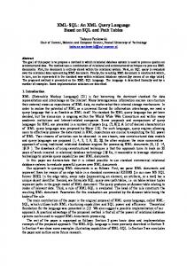
We performed different experiments based upon a number of interesting and uninteresting clips. In our experiments, to measure the correctness and validation of our approach, we obtained our measurements based on what is described in the database. In other words, if hair type is not stored in the database, the user does not browse clips based on hair type. It is not possible to check the correctness of our method by testing on missing information in the database. The user is provided a set of clips that includes both interesting and uninteresting clips. The user browses a subset of these clips; and interesting and uninteresting sets are generated based on the user browsing feedback. Then the user tells the expert what his or her intended query was. The expert has a good knowledge of the database which enables the expert to set up the correct query from the database. The expert builds the query and then submits it to the database system. The clips that are retrieved from the database are correct clips. We do not need more than one expert as in other traditional content-based retrieval systems to determine ground-truth, since the retrieval from the database is objective (not subjective). We experimented with how the number of interesting and uninteresting clips affect the retrieval. We assumed the user is likely to view 10 clips (partially or completely) on the average. The ratio of correctly retrieved clips for (10 interesting, 0 uninteresting clips), (8 interesting, 2 uninteresting clips), (6 interesting, 4 uninteresting clips), (4 interesting, 6 uninteresting clips), and (2 interesting, 8 uninteresting clips) are displayed in Fig. 1, 2, 3, 4, and 5, respectively. This ratio shows the ratio

25

Figure 1: Performance for 10 interesting and 0 uninteresting clips.

Figure 2: Performance for 8 interesting and 2 uninteresting clips. of retrieved clips to total correct clips. This ratio becomes 1 (meaning all correct clips are retrieved) as the threshold is lowered. Note that I-Quest returns only correct clips in the experiments. I-Quest will not return irrelevant clips. This shows that our system is able to estimate what the user is looking for. The ratio of correctly retrieved clips for threshold θ = 0.85 are 1.0, 0.958, 0.875, 0.333, and 0.0416 in the cases of 10, 8, 6, 4, and 2 interesting clips, respectively. These results show that as the number of interesting clips increases, it is possible to achieve high performance values at higher thresholds. The reason for having performance (ratio) values when the number of interesting clips is low is that there might be more common attributes in a few interesting clips than is the case for many interesting clips. In other words, what is common in two interesting clips is less likely to be common in four interesting clips. These results also show that the expected clips can be retrieved when at least 2 interesting clips are provided to the system.

26

Figure 3: Performance for 6 interesting and 4 uninteresting clips.

Figure 4: Performance for 4 interesting and 6 uninteresting clips. The size of the database does not affect or degrade the correctness of our approach. Our method considers only clips in the interesting and uninteresting sets to determine what needs to be retrieved from the database. 5.2.2

Subjective Evaluation

We have also performed subjective evaluation of our system using graduate and undergraduate students of the University of Alabama in Huntsville. The user browses a set of clips from the database and the interesting and uninteresting sets are computed after the browsing is completed. We asked the users to be consistent during browsing. The user has a query in his or her mind and stays loyal to the query during browsing. For example, if the clip is not relevant, the user should

27

Figure 5: Performance for 2 interesting and 8 uninteresting clips. not watch it completely. After processing the sets and calculating the relevances, our system shows the results with the clips that have high relevance on the top and low relevance on the bottom. As long as the user is consistent, our system always returns only the relevant clips. The ratio of correctly retrieved clips is usually obtained as 1 when the threshold is at least δ. At the end of each experiment, we made a survey whether the students are satisfied with the output of our approach or not. Our method satisfied the students approximately for 97.5% of experiments. 5.2.3

Discussion on Performance Results

In our early studies, we computed the precision and recall values. Our precision/recall values are higher than expected for information retrieval systems. In information retrieval systems, it is unlikely to get a high precision with a high recall. In most cases, as precision increases, recall decreases or vice versa. Our system builds a query and executes this query on the database. If the query is created correctly, the precision and recall will be both 1.0. Such precision and recall values are almost impossible in other information retrieval systems. It is not fair to say that our system is better than other information systems. There are two major differences between our system and other retrieval systems; these are identified in the title of our paper: query structuring and semantic video database. Our goal is to build the query correctly. If the query is built correctly, the user has the correct result. The traditional database systems do not sort the results. However, our system computes relevance and provides a sorted list of the results. Low-level feature extraction and mapping these features to high-level features are one of the important points of our system. We still work on automating this step. However, when lowlevel features are mapped to high-level features, they are maintained as high-level features in the

28

database. I-Quest works on high-level features. However, I-Quest does not support queries such as find the video clips where the trajectory of a ball is similar to a specific user-drawn trajectory. For such queries, low-level features are definitely a big contribution to retrieval accuracy. We again illustrate this on tennis videos. Low-level features are an important part of our future system. They are used to generate high-level features and for retrieval based on features where it is hard to store low-level features in a traditional relational database.

5.3

Comparison with Previous Approaches

In this section, we point out the limitations of the previous approaches. We compare our algorithm specifically with the inter-ranking algorithm [19] and the personalization algorithm in [25]. The inter-ranking algorithm explicitly treats the interesting and uninteresting sets that are selected by the user. On the other hand, the keywords that are related to the browsed clips are regarded interesting and the rest in non-browsed clips are considered as uninteresting. In [25], a hierarchical representation of video clips is considered and the weight of a keyword is determined depending on the fraction of a video clip watched by the user and whether the keyword appears in the child segments or not. The weight of a keyword is incremented by a value (depending on the portion of a clip watched by the viewer) and reduced by a multiplying a constant between 0 and 1 if a keyword is related to unwatched clip. In [19], the weight of an attribute is determined by the number of different values for the attribute in the interesting (or uninteresting) set. They ignore the frequency of attribute values. Consider two scenarios in which there are 10 clips for two attribute values. In the first case, the frequency of attributes are 9 and 1; and in the second case their frequencies are 5 and 5. Since the number of different attribute values is the same, the weight of the attribute is considered the same regardless of the frequency of the values. Even there is a match for the attribute values with the lowest appearance, those clips have scores same as the scores of clips having the frequent item. 5.3.1

Comparison with the inter-ranking algorithm.

The inter-ranking algorithm determines the weight of attributes by checking the diversity of attribute values. If the diversity of attribute values is low for an attribute, that attribute is given more weight than the others. The (positive) relevance of a clip is determined by maximum similarity to any one of the selected clips. Consider the set of clips that are chosen as interesting in Table 6 and uninteresting in Table 7. These sets indicate that the user has strong interest in (Beckham, Goal) than any other clip, so the relevance of clips having (Beckham, Goal) should be more than the others. The inter-ranking

29

Clip No c1 c2 c3 c4

Player Beckham Beckham Beckham Ronaldo

Event F oul Goal Goal Goal

Table 6: Interesting Clips. Clip No c5

Player N istelroy

Event Corner

Table 7: Uninteresting Clips. algorithm ignores the frequency of attribute values and puts emphasis on the diversity of attribute values. For example, the diversity for player is 2 (2 players are listed) for the interesting set. The same case applies for the event. The number of appearances of (Beckham, Goal) does not effect the computation of a relevance of a clip. Our ranking algorithm gives importance to the frequency of attribute values as well. The clips having (Beckham, Goal) will have higher ranking than other clips (Table 8). Our algorithm has three advantages over the inter-ranking algorithm. Firstly, it gives the highest relevance to clips that occur frequently in the interesting set. (Beckham, Goal) is rated higher than other player, event pairs. This is not the case with the inter-ranking algorithm. Secondly, our method can deal with clips that are browsed incorrectly. The clip c4 has a different player than the rest of the clips in the interesting set. However, its score (c8 ) by the inter-ranking algorithm is the same as the clip c6 . Thirdly, our method provides an ordering (ranking) among different clips. On the other hand, the inter-ranking algorithm assigns the same relevance to many clips. A clip (c10 ) that is not watched at all has the same score as clips c11 , c12 , c13 in the inter-ranking algorithm. The ranking of the clips is important especially if there are many clips that match the Clip No c6 c7 c8 c9 c10 c11 c12 c13 c14

Player Beckham Beckham Ronaldo Ronaldo Guiza Beckham Ronaldo N istelroy N istelroy

Event Goal F oul Goal F oul Out Corner Corner F oul Corner

Inter-ranking score 1 1 1 0.75 0.5 0.5 0.5 0.5 0

Table 8: Clip Scores. 30

I-Quest score 0.8 0.67 0.67 0.53 0 -0.81 -0.813 -0.813 -0.92

Clip No c15 c16 c17 c18

Player Beckham Beckham Beckham Beckham

Attr1 A11 A11 A21 A11

Attr2 A12 A12 A22 A12

Attr3 A13 A13 A23 A13

Attr4 A14 A14 A24 A14

Table 9: Interesting Clips. Clip No c19

Player Ronaldo

Attr1 A41

Attr2 A42

Attr3 A43

Attr4 A44

Table 10: Uninteresting Clips. same properties. Our algorithm is able to provide a good ranking of the results. Consider another example where the user is interested in the player Beckham but the database has 4 more attributes per clip. It is likely that there may be some coincidence between the last 4 attributes. Consider the set of interesting clips in Table 9 and uninteresting clips with Table 10. Table 11 provides the scores of two clips. The inter-ranking algorithm cannot determine that Beckham is the focus of the query. Clip c20 gets a very low score by inter-ranking algorithm since it also had some matching attributes with the clip in the uninteresting set. However, our method is able to provide a good score to clip c20 . The inter-ranking algorithm gives a higher rank to clip c21 since it had a good match to one of the clips in the interesting set. However, the player ’Jack’ is not the user’s interest. The limitations of the inter-ranking algorithm can be summarized as follows: 1. Unsatisfactory ranking (many clips have the same relevance). 2. Relevance is determined based on the similarity to the most similar object (the number of appearances of values have little to no effect on the relevance). 3. All attributes are considered to have effect on the relevance computation. 5.3.2

Comparison with the personalization algorithm.

The personalization algorithm implicitly groups clips (actually keywords) as interesting and uninteresting. The keywords of browsed clips are interesting and the rest are uninteresting. In the Clip No c20 c21

Name Beckham Jack

Attr1 A41 A21

Attr2 A42 A22

Attr3 A43 A23

Attr4 A44 A24

Inter-ranking score 0.27 0.83

Table 11: Clip scores. 31

I-Quest score 0.800 0.53

Clip No c22 c23

Player Beckham Beckham

Event Corner Corner

Team Manchester United Manchester United

Table 12: Interesting Clips. Clip No c24 c25

Player Ronaldo Rooney

Event Corner Corner

Team Manchester United Manchester United

Table 13: Uninteresting Clips. personalization algorithm, the weights of keywords (or attribute values) are incremented by a computed value if they appear in a browsed clip; otherwise the weight of a keyword is reduced by multiplying a coefficient between 0.9 and 1. However, the personalization algorithm does not provide a good solution for common keywords that appear in browsed and non-browsed clips. Basically, if a keyword appears in a browsed clip, its weight is increased regardless of that attribute value appears in a non-browsed clip or not. Consider an example where the user has interest in the player Beckham but not in the event or the team. The user identifies no interest in team and event through the set of uninteresting clips. Assume that the clips in Table 12 are browsed clips and the others in Table 13 are not browsed. Table 14 provides the scores of various clips. In this case, the personalization algorithm cannot determine that the most important attribute is the player. Because of that, (Nistelroy, Corner, Manchester United) clip gets a higher rank than clip c9 that has Beckham as a player. A good set of interesting clips should also have player Beckham with Real Madrid to emphasize that the player is the interesting attribute. The personalization algorithm treats every attribute value that appears in an interesting set as important. Actually, their test data set has only two attributes (player, event). In their data set, all attributes are important for the user. However, in reality in annotated databases there are usually more than 2 attributes defined for each clip and not necessarily all Clip No c26 c27 c28 c29 c30 c31 c32

Player Beckham N istelroy Beckham Beckham N istelroy N istelroy Beckham

Event Corner Corner Corner Goal Goal Corner Goal

Team Manchester United Manchester United Real Madrid Manchester United Manchester United Real Madrid Real Madrid

Personalization score 6 4 4 4 2 2 2

Table 14: Clip Scores.

32

I-Quest score 0.84 0 0.84 0.84 0 0 0.84

Clip No c1 c2 c3 c4

Attribute A a1 a1 a1 a1

Attribute B b1 b1 b2 b2

Attribute E e1 e2 e2 e3

Table 15: A sample set of relevant clips for probability analysis. attributes are important for the user. Our methodology provides a way of eliminating irrelevant attributes and they have less effect on the ranking.

5.4

Probabilistic Analysis

The set of clips that are browsed by the user and the number of browsed clips play an important role in the retrieval performance of I-Quest. The set of clips in the uninteresting set helps I-Quest eliminate some uninteresting attributes. If the user does not browse any uninteresting clip, the elimination of uninteresting attributes is difficult since these attributes appear in interesting clips. In this section, we consider this difficult case where the user browses only interesting clips. In this sense, browsing an interesting clip is equivalent to selecting a clip. The performance of I-Quest can be degraded if the selected clips are very similar to each other with respect to uninteresting attributes. In such cases, it is possible that retrieval precision may be lower than the precision in the aforementioned experiments. For example, the user may be interested in video clips of actors having blue eyes. If the actors in the interesting clips have also the same hair style, then our system will also retrieve the clips of other actors with that hair style. Assume that the user browses k clips out of n relevant clips in the database. Consider all relevant clips (i.e. attribute A = a1 ) that are provided in Table 15 where n = 4 and k = 2. If the user browses clips c1 and c2 as interesting, I-Quest determines that the user is interested in both attribute values a1 and b1 . In the same way, if the user browses clips c2 and c3 as interesting, I-Quest determines that the user is interested in both attribute values a1 and e2 . The combination of selecting k clips out of n clips is C(n, k). In this case, the combination is C(4, 2) = 6. Let nk be the number of all groups of k clips among n relevant clips having at least one common attribute value apart from the interesting attribute. The probability of selecting a good set of clips can be computed as P (good selection|N = n, K = k, N K = nk ) = 1 −

nk C(n,k)

(5)

where N , K, and N K are random variables to represent the number of relevant clips, the number of selected clips, and the number of groups of clips having a common attribute value, respectively. 33

The probability of selecting a good set of clips is 1-(2/6) for the previous example. If the user selects 3 clips, the probability of selecting a good set of clips is 1. In other words, whatever the 3 clips are browsed as interesting, the query will be created properly. The set of dependencies among attributes theoretically originates from the functional dependencies of the database. However, practically, that may not be true due to the distribution of attribute values. All attributes of a clip need to be considered for computing probability. However, the appearances of attribute values are not independent of each other. Therefore, the probability of having the same value for an attribute is not independent from the appearance of a value for another attribute. We consider each attribute one at a time. The following probability includes good selection of attributes considering only one attribute, where N , K, and M are random variables, to represent the number of relevant clips, the number of selected clips by the user, and the average number of appearances for an attribute value among N relevant clips. Note that n/m is the different number of attribute values for the relevant clips: P (good selection|N = n, M = m, K = k) = = = =

n/m

1 − Σi=1 P ermutation(m,k) nk n/m m! 1 − Σi=1 nk ∗k! n m! 1− m nk ∗k! 1 − n((m−1)! k−1)∗k!

(6)

To analyze the performance of our system, we provide two sample cases. In the first case, we assume that an attribute value appears a specific number of times whereas the remainder of the attribute values are different from each other. This number is represented with h. Figure 6 displays the probability of good selection with different h and k values. It can be seen that as k increases, the probability of good selection increases. In our original experiments, we asked the user to select 10 clips. If the user selects 10 clips, the probability of selecting a bad set of clips is extremely low (0.00432) even for the same 60 values (h = 60) out of n = 100 values. In the second case, we changed the number of attribute values based on an average number of appearances (m). We assumed that each attribute value has an equal chance of appearance. In Figure 7, m represents the average number of times a value may appear. If m = 2, there are 64 different values for n = 128. It can be seen that the probability of selecting a good set of clips is close to 1 for m ∈ {2, 4, 8, 16, 32}. This probabilistic analysis shows that if the user watches more clips, the probability of getting only the expected clips becomes higher. In the same way, if an attribute value is not dominant (or frequent), the probability of getting only the expected clips also increases. It can be noted that with selection of 10 clips by the user, the probability of retrieving incorrect clips is almost 0.

34

Figure 6: Probability of good selection for n=100 with specific number of the same attribute value.

5.5

Discussion

We wish to point out two important points about our results and system. • If a user does not have a specific query in mind, the user is likely to browse the clips randomly. Random browsing does not retrieve any meaningful video clips. Random browsing is equivalent to selecting relevant and irrelevant images randomly in an image retrieval system based on relevance feedback. Users of our system have queries in their minds and are loyal to their queries while browsing. We provide a guide before browsing for how a user should behave for interesting and uninteresting clips. • When a user connects to our system, a session is created for the user as in relevance feedback on any client/server systems. The clip identifiers of interesting and uninteresting clips for a user are stored in the database. Six sets are generated using database queries based on two tables (interesting and uninteresting) having at most 10 tuples (clips) practically. Definite relevance is computed with one pass on definite sets. For the computation of probable and contingent relevances, the number of times the values appear for each attribute are computed for each of the probable and contingent sets. These computations are minor with respect to retrieval of clips from the database. Having a session per user as in relevance feedback systems is a must to serve multiple users simultaneously.

35

Figure 7: Probability of good selection for n=128 with different number of attribute values.

6

Conclusion

In this paper, we have shown a method to extract user interest based on the user browsing of query results. I-Quest can rank results with respect to a set of interesting and uninteresting sets obtained from user browsing. The main contribution of I-Quest is its success when a template object cannot be generated from the set of interesting and uninteresting clips as discussed in this paper. I-Quest also helps the user access the data when he or she is unable to formulate the query properly. We have promising results from our experiments. The current work can be extended in several ways: First, we consider the possibility of incorrect user browsing and then improve our algorithm when the user accuracy is low. Second, in our system, the application determines what type of browsing should be followed by the user to identify interesting and uninteresting clips. We wish to remove this restriction in two ways: a) allow the user to define his or her browsing behavior, or b) build a classifier to identify how the user reacts to interesting and uninteresting clips and use this classifier in the identification of interesting and uninteresting clips. Third, we could evaluate the implicit browsing feedback [36, 37] rather than the explicit feedback. In other words, the user does not need to know how the system performance can be improved. We would like to automatically classify the interesting and uninteresting clips from a set of clips that are browsed by the user. Acknowledgment. We would like to thank Parthan Ulagarakshagan for implementing the baseball video database application.

36

References [1] J. M. Martinez, R. Koenen, F. Pereira, Mpeg-7: The generic multimedia content description standard, part 1, IEEE Multimedia 9 (2) (2002) 78–87. [2] J. M. Martinez, Mpeg-7: Overview of mpeg-7 descrition tools, part2, IEEE Multimedia 9 (3) (2002) 83–93. [3] M. Ortega-Binderberger, S. Mehrotra, Handbook of Video Databases: Design and Applications, CRC Press, 2003, Ch. Relevance Feedback in Multimedia Databases, pp. 511–535. [4] P.-Y. Yin, K.-C. Chang, A. Dong, Integrating relevance feedback techniques for image retrieval using reinforcement learning, IEEE Trans. Pattern Anal. Mach. Intell. 27 (10) (2005) 1536– 1551, fellow-Bir Bhanu. [5] I. J. Cox, M. L. Miller, T. P. Minka, P. N. Yianilos, An optimized interaction strategy for bayesian relevance feedback, IEEE Conference on Computer Vision and Pattern Recognition (CVPR’98). [6] Y. Rui, T. Huang, S. Mehrotra, Content-based image retrieval with relevance feedback in mars (1997). URL citeseer.nj.nec.com/rui97contentbased.html [7] Y. Rui, T. S. Huang, M. Ortega, S. Mehrotra, Relevance feedback: A power tool in interactive content-based image retrieval, Special issue on Segmentation, Description, and Retrieval of Video Content, IEEE Transactions on Circuits and Systems for Video Technology 8 (5) (1998) 644–655. [8] Y. Rui, T. S. Huang, S. Mehrotra, M. Ortega, Automatic matching tool selection via relevance feedback in mars, Proceedings of the Second International Conference on Visual Information Systems (1997) 109–116. [9] Y. Rui, T. S. Huang, S. Mehrotra, M. Ortega, A relevance feedback architecture in contentbased multimedia information retrieval systems, Proceedings of IEEE Workshop on ContentBased Access of Image and Video Libraries, in conjunction with CVPR’97 (1997) 82–89. [10] G. Salton, C. Buckley, Improving Retrieval Performance by Relevance Feedback, Journal of the American Society for Information Science 41 (4) (1990) 288–297. [11] L. Taycher, M. La Cascia, S. Sclaroff, Image digestion and relevance feedback in the imagerover www search engine, Proceedings of International Conference on Visual Information. 37

[12] R. Wang, M. Naphade, T. Huang, Video retrieval and relevance feedback in the context of a post-integration model, in: 2001 IEEE Fourth Int. Workshop on Multimedia Signal Processing, 2001, pp. 33–38. [13] P. Munesawang, L. Guan, Adaptive video indexing and automatic/semi-automatic relevance feedback., IEEE Trans. Circuits Syst. Video Techn. 15 (8) (2005) 1032–1046. [14] M. Ortega, Y. Rui, K. Chakrabarti, K. Porkaew, S. Mehrotra, T. S. Huang, Supporting ranked boolean similarity queries in MARS, IEEE Transactions on Knowledge and Data Engineering 10 (6) (1998) 905–925. [15] G. Salton, E. Fox, H. Wu, Extended Boolean Information Retrieval, Communications of the ACM 26 (12) (1983) 1022–1036. [16] Y.-S. Chen, C. Shahabi, Yoda, an adaptive soft classification model: content-based similarity queries and beyond, Multimedia Systems 8 (2003) 523–535. [17] L. Zadeh, Similarity Relations and Fuzzy Orderings, Information Sciences (1971) 177–200. [18] L. Wu, C. Faloutos, K. Sycara, T. Payne, D. R. McCarthy, FALCON: Feedback adaptive loop for content-based retrieval, in: Proceedings of the 26th International Conference on Very Large Data Bases, Cairo, Egypt, 2000, pp. 297–306. [19] Y. Zhang, X. Zhang, C. Xu, H. Lu, Personalized retrieval of sports video, in: MIR ’07: Proceedings of the international workshop on Workshop on multimedia information retrieval, ACM, New York, NY, USA, 2007, pp. 313–322. [20] J. Shao, Z. Huang, H. T. Shen, X. Zhou, E.-P. Lim, Y. Li, Batch nearest neighbor search for video retrieval, Multimedia, IEEE Transactions on 10 (3) (2008) 409–420. [21] C. Fellbaum (Ed.), WordNet: An Electronic Lexical Database (Language, Speech, and Communication), The MIT Press, 1998. [22] C. G. M. Snoek, M. Worring, D. C. Koelma, A. W. M. Smeulders, A learned lexicon-driven paradigm for interactive video retrieval, IEEE Transactions on Multimedia 9 (2) (2007) 280– 292. [23] C. Xu, J. Wang, H. Lu, Y. Zhang, A novel framework for semantic annotation and personalized retrieval of sports video, Multimedia, IEEE Transactions on 10 (3) (2008) 421–436.

38

[24] X. He, W.-Y. Ma, M. Li, H.-J. Zhang, Learning a semantic space from user’s relevance feedback for image retrieval., IEEE Trans. Circuits Syst. Video Techn. 13 (1) (2003) 1032–1046. [25] N. Babaguchi, K. Ohara, T. Ogura, Learning personal preference from viewer’s operations for browsing and its application to baseball video retrieval and summarization, Multimedia, IEEE Transactions on 9 (5) (2007) 1016–1025. [26] M. S. Lew, N. Sebe, C. Djeraba, R. Jain, Content-based multimedia information retrieval: State of the art and challenges, ACM Trans. Multimedia Comput. Commun. Appl. 2 (1) (2006) 1–19. [27] S. Hoi, M. Lyu, A multimodal and multilevel ranking scheme for large-scale video retrieval, Multimedia, IEEE Transactions on 10 (4) (2008) 607–619. [28] D. Heesch, P. Howarth, J. Magalhaes, A. May, M. Pickering, A. Yavlinsky, S. Ruger, Video retrieval using search and browsing, in: Proceedings of TRECVID2004, 2004. [29] Y. Mezaris, H. Doulaverakis, S. Herrmann, B. L. N. O’Connor, I. Kompatsiaris, G. M. Strintzis, Combining textual and visual information processing for interactive video retrieval: Schema’s participation to trecvid2004., in: Proceedings of TRECVID2004, 2004. [30] MPEG7:XM, http://www.lis.ei.tum.de/research/bv/topics/mmdb/e mpeg7.html (2006). [31] X. Mu, Content-based video retrieval: does video’s semantic visual feature matter?, in: SIGIR ’06: Proceedings of the 29th annual international ACM SIGIR conference on Research and development in information retrieval, ACM Press, New York, NY, USA, 2006, pp. 679–680. [32] T. Syeda-Mahmood, D. Ponceleon, Learning video browsing behavior and its application in the generation of video previews, in: Proceedings of the 9th ACM international conference on Multimedia, Ottawa, Canada, 2001, pp. 119–128. [33] A. Hauptmann, R. Yan, W.-H. Lin, M. Christel, H. Wactlar, Can high-level concepts fill the semantic gap in video retrieval? a case study with broadcast news, Multimedia, IEEE Transactions on 9 (5) (2007) 958–966. [34] J. Allen, Maintaining Knowledge about Temporal Intervals, Communications of ACM 26 (11) (1983) 823–843. [35] R. Elmasri, S. B. Navathe., Fundamentals of Database Systems, Addison Wesley, 2006, fifth edition. 39

[36] X. Shen, B. Tan, C. Zhai, Context-sensitive information retrieval using implicit feedback, in: SIGIR ’05: Proceedings of the 28th annual international ACM SIGIR conference on Research and development in information retrieval, ACM, New York, NY, USA, 2005, pp. 43–50. [37] D. Kelly, N. J. Belkin, Display time as implicit feedback: understanding task effects, in: SIGIR ’04: Proceedings of the 27th annual international ACM SIGIR conference on Research and development in information retrieval, ACM, New York, NY, USA, 2004, pp. 377–384.

40