Jan 21, 2008 - model. A non-integer Ctnn is composed of a neural network and a non integer ... Keywords: Neural networks, Non integer integrator, Non linear ...
Author manuscript, published in "lFAC Workshop on Fractional Differentiation and its Applications, Porto : Portugal (2006)"
IDENTIFICATION OF NON LINEAR FRACTIONAL SYSTEMS USING CONTINUOUS TIME NEURAL NETWORKS Fran¸ cois Benoˆıt-Marand ∗ Laurent Signac ∗ Thierry Poinot ∗ Jean-Claude Trigeassou ∗
hal-00211783, version 1 - 21 Jan 2008
∗
Laboratoire d’Automatique et d’Informatique Industrielle Bˆ atiment de M´ecanique 40, avenue du recteur Pineau 86022 Poitiers, France
Abstract: Fractional systems allow us to model the processes governed by a diffusive equation. The simulation of such processes can be realized by using a non integer integrator. The aim of this paper is to estimate, in the time domain, both the non integer derivative order and the physical law of a non linear fractional system. To achieve this goal, we use Continuous Time Neural Networks. Ctnn are dynamical neural structures that differ from the classical recurrent neural networks on the use of integrator blocks rather than delay blocks. This difference allows us to access the physical law of the system rather than only having a black box model. A non-integer Ctnn is composed of a neural network and a non integer integrator. The identification stage –which consists in finding the good parameters for the neural network and for the integrator block– will be performed by using an output error identification. At the end of the procedure, a model reduction stage can be performed in order to revert from the neural network to a more realistic expression of the physical law of the process. To illustrate the method we’ll give some simulation results. Keywords: Neural networks, Non integer integrator, Non linear fractional systems, Output error identification
1. INTRODUCTION Fractional systems are used to model the physical processes governed by a diffusive equation and have already been used in many different fields like thermics (Battaglia, 2002; Cois, 2002), electrochemistry (Lin et al., 2000a) or electromagnetism (Lin et al., 2000b; Reti`ere and Ivanes, 1998). The works in progress at the Laii∗ are based on the definition of a non integer integrator (Lin, 2001) that allows us to simulate linear and non linear fractional systems (Poinot and Trigeassou, 2004). In this paper, we will focus on the modeling and the identification of non linear fractional systems by using neural networks.
An original method using neural networks has already been developed in the case of non linear integer systems (Benoˆıt-Marand et al., 2004). This method, referred to as Ctnn, combines a neural network with an integer integrator block. Contrary to the classical recurent neural networks, that use delay blocks and only give a black box model of the process, Ctnn, by separating the non linear static part of the process (the neural network) from the dynamical one (the integrator block), allows us to access the physical law of the process. In this article, we will show how, by using a non integer integrator in the Ctnn structure,
it is possible to extend the previous method to fractional systems. During the identification stage, we will not only have to estimate the parameters of the network which characterize the system’s law but to estimate the derivative order of the system too. These parameters will be found by using an output error identification technique with temporal data. First, we point out the definition of the non integer integrator and its state space representation. Then we show the principles of Ctnn and their extension to fractional systems. Then, the identification stage is exposed. Finally, we illustrate our method by simulation results.
20 dB/decade and to a phase equal to −n × 90o for any frequency. This theoretical frequency response can be approximated on a limited band [ωb , ωh ] (according to the desired accuracy) using cascade phase lead filters (Oustaloup, 1995), associated with an 1/s integrator (Poinot and Trigeassou, 2003). Consider the following approximation of the theoretical non integer integrator (Lin, 2001) which corresponds to the Bode diagram on figure 1: N
G Y1+ Iˆn (s) = s i=1 1 +
s ωi′ s ωi
(3)
ρ dB
2. FRACTIONAL SYSTEMS AND NON INTEGER INTEGRATOR
hal-00211783, version 1 - 21 Jan 2008
log ω
ωh
log ω − n × 90° −90°
(1)
This differential equation, generally non-linear, may be integrated with the help of an operator I(s) = 1s , which performs time integration of dy(t) dt (in order to give y(t) at its output). Practically, we use a numerical integrator (Euler,RungeKutta 4,...) instead of an analog one ( 1s ).
Fig. 1. Bode diagram of Iˆn (s) Its frequency response is a suitable approximation of the theoretical one : • The intermediate zone (ωb < ω < ωh ) corresponds to the non integer behavior of the integrator, characterized by n. • For low and high frequencies, the behavior of the integrator is conventional, with n = 1.
Then, let us consider the fractional differential equation (n is the non integer derivative order): dn y (t) = f (u (t) , y (t)) dtn
ωb
θ
Let us consider the following integer differential equation (u (t) and y (t) are the input and the output of the system): dy (t) = f (u (t) , y (t)) dt
ωh
ωb
2.1 Simulation of fractional systems
(2)
Finally, given N , n, ωb , ωh , the operator introduced by (3) is completely defined by the following relations 1 :
Assume that a fractional integrator In (s) = s1n is n available (its input is equal to d dty(t) so that its n output is equal to y(t)).
′
ω1 = ωb , ′
ωi = α ωi ,
Thus, In (s) generalizes to fractional systems the previously presented simulation principle. As a conclusion, integration of fractional systems simulation essentially relies on the definition of a fractional integrator, which will be a generalization of the conventional one. Notice that this technique applies either to linear or to non-linear fractional systems, which is the main interest of the non-integer operator.
v(t)
′
ωi+1 = η ωi , x1 (t)
G s
v(t) =
s ′ ω 1 1+ ωs 1
1+
dn y(t) dtn
ωu =
√
ωb ωh ,
n=1− s ′ ω N 1+ ωs N
1+
···
ln α ln α η
(4)
xN +1 (t)
xN +1 (t) = y(t)
Fig. 2. Iˆn (s) block diagram Using the block diagram shown in figure 2, Iˆn (s) can be described by the following state-space representation (Poinot and Trigeassou, 2003):
2.2 Definition of the non integer integrator The ideal fractional integrator is defined by using the transfer function In (s) = s1n which corresponds to a magnitude’s slope equal to −n ×
ωN = ωh ,
·
x = A∗ x + B ∗ v
(5)
In (3) G is defined so that� the magnitude of Iˆn (s) is n equal to the magnitude of 1s for the frequency ωu .
1
where
A∗ = M −1 A, B ∗ = M −1 B, B T = [Gn 0 · · · 0], 0 0 ··· 0 1 0 ··· 0 . . . . ω −ω1 −α . . . . . ,A= 1 M = .. . . . . .. . . . . . . . . 0 0 . . 0 · · · ωN −ωN 0 · · · −α 1
3. CONTINUOUS TIME NEURAL NETWORKS
hal-00211783, version 1 - 21 Jan 2008
There are two main approaches to simulate dynamical systems with a neural network. The first one consists in using dynamical units (continuous time neurons). Many models have been proposed (Hopfield, 1982; Pearlmutter, 1995; matopou los et al., 1995) and complex processes have been simulated or controlled by such networks. Nevertheless, the physical law of the process can not be extracted because dynamical and static components of the model are not separated. The second approach is based on the use of a static net associated with an external dynamical component. Delay blocks (figure 3) may be used (Narendra and Levin, 1997) in order to obtain a discrete representation of the system: yˆk+1 = g(uk , yˆk ) where g is the function computed by the net. z −1 ybk uk
Neural ybk+1 Network
d the continuous equation of the system: dy(t) = dt g (u(t), yˆ(t)) where g is the function computed by the net. Obviously, we can separate the static part of the process (the function computed by the net) from the dynamical one (Benoˆıt-Marand et al., 2005). By definition the net gives us direct access to the physical law of the simulated process. The idea is simple but powerful. Indeed, we need to adapt neither the net structure nor the principles of the identification procedure if we change the integration method. In particular, the integrator may be a fractional integrator. yb(t)
u(t)
dt
yb(t)
4. OUTPUT ERROR IDENTIFICATION 4.1 Presentation In the following, we will consider a Ctnn dedicated to single input single output fractional systems. We use the single hidden layer static net described figure 5 followed by a non integer integrator (figure 6). Adjustable parameters of the model, called θ, are the 4Nc parameters of the net which characterize the physical law and parameter α characterizing the derivative order of the fractional integrator. θ T = [w1,1 · · · w3,Nc
y
w2,i w3,i
u
P
n1
P
nj
tanh
tanh
bi P
s
1 bN c P
nN c
tanh
Fig. 5. The static neural network used in the Ctnn System
y∗
+ −
u
Neural s = Network
d dn y dtn
In
dy(t)
Suppose dt = f (u(t), y(t)) = au(t) + by(t), then the function computed by the static net is not equal to f but to eaT x(t) + ab (1 − e−aT )u(t), and in the non linear case we do not have such relation to revert to the physical law.
α]
b1 · · · bNc
b1 w1,i
We proposed a method (Benoˆıt-Marand et al., 2004; Benoˆıt-Marand et al., 2005), referred to as Ctnn: we use a static feed-forward neural network followed by a continuous integration method (figure 4). Our model is directly related with 2
Z
c dy
Fig. 4. A Continuous Time Neural Network Ctnn
Fig. 3. Discrete time neural network Such models have been successfully investigated in process control (Narendra, 1992) but don’t give direct access to the physical law of the system 2 . An enhanced design has been proposed (Wang and Lin, March 1998) to obtain a discretization of the process using the Runge-Kutta 4 (Rk4) scheme: the net approaches the physical law of the system with an high accuracy. Nevertheless, by using a discrete representation of the process, the whole neural structure and the identification procedure have to be adapted according to the desired accuracy (Euler, Rk4) or to the desired task.
Neural s = Network
Fig. 6. Output error identification
yb
The aim of the identification stage is to find θ∗ which minimizes the following criterion 3 :
J=
K X
k=1
(yk∗ − ybk )2 =
k=K X
using the non integer integrator used in the Ctnn model. The computation of ∂s(t) ∂θp is performed with the well-known back propagation algorithm (Cun, 1985; Rumelhart et al., 1986) 4 :
e2k
k=1
∂s(k) = tanh(ni (k)) ∂bi ∂s(k) = ri (k) · tanh′ (nj (k)) · bj ∂wi,j
4.2 The Levenberg-Marquardt algorithm We solve the previous optimization problem using the iterative Levenberg-Marquardt algorithm (Marquardt, 1963; Hagan and Menhaj, 1994):
∂s(t) ∂b y(t)
The value of e θ + λI) θ i+1 = θi + ∆θ with ∆θ = (H
hal-00211783, version 1 - 21 Jan 2008
−1
Jθ′
e θ is the Jθ′ is the gradient of J with respect to θ, H pseudo-hessian matrix of J with respect to θ, and λ is a control parameter of the algorithm. Jθ′ and e θ are computed using the following relations: H � ∂b yk = −2 ek · ∂θ k=1 � K � h i X ∂b yk ∂b yk e H =2 · ∂θj ∂θl j,l k=K X�
Jθ′
is easy to compute:
i=N Xc ∂s(t) w1,i · tanh′ (ni (t)) · bi = ∂b y (t) i=1
4.4 Calculus of the sensitivity function associated with the parameter of the non integer integrator y ˆ(t) we derivate the To evaluate σα (t) = ∂∂α state space representation (5) with respect to α. Extending the state space vector with x(N +1+i) (t) = ∂xi (t) ∂α , we obtain the following modified state space representation:
k=1
Let’s define the value of the sensitivity function of yk . the parameter p for the sample k as σp (k) = ∂∂θb p To solve the optimization problem we have to compute this value for all p and all k.
·
x = C ∗ x + D∗ v where:
�
� dn yb (θ, u(t), yb(θ, t)) dtn
∂ dn σp (t) = dtn ∂θp ∂ (s(θ, u(t), yb(θ, t)) = ∂θp y(t) ∂s(t) ∂s(t) ∂b + · = ∂θp ∂b y(t) ∂θp ∂s(t) ∂s(t) = + · σp (t) ∂θp ∂b y(t)
i
∂f σα (t) ∂ yˆ(t)
v T = f (u(t), yˆ(t), θ)
4.3 Calculus of the sensitivity functions associated with the parameters of the neural network This calculus is referred to as dynamic back propagation (Narendra and Parthasarathy, March 1991) and has already been successfully used in the case of integer Ctnn (Benoˆıt-Marand et al., 2004). It can directly be extended to fractional Ctnn (0 < n < 1). We simply write:
h
D=
�
C ∗ = R−1 C yˆ(t) = x(N+1) (t)
�
D1 0 D2 D1
R=
�
(6)
D ∗ = R−1 D σα (t) = x(2N+2) (t)
�
M 0 R1 M
C=
�
A 0 C1 A
�
M , A are the matrices defined in (5). D1 , D2 (vectors of size N + 1) and R1 , C1 (square matrices of size N + 1) are defined as follows: i h � � ∂G T T =
D1
R1 =
0
−1 ∂ω1 ∂α
G 0 ···
. .
. .
. . .
.
. −1 0
∂ωi
= ωb
∂α ∂η
∂α
=
h
C1 =
= αη
ωh ωb
=
D2
∂ωi−1 ∂α
i N1−1 �
∂α
0 ···
0
∂ω1 ∂α
−
∂ω1 ∂α .
+ ωi−1 N
1−N
�
.
.
h
. . . ∂ωN
∂α ∂η η+α ∂α
2N −1
i
−
∂ωN ∂α
Finally, let’s calculate ∂G ∂α . G is such that magnitudes jω 1+ ω ′ Q 1 G k and (jω) of Iˆn (ω) = jω n are equal if 1+ jω ω = ωu . As a consequence: 4
3
K is the size of the data set
α 1−N
ωk
So, the sensitivity functions associated with the neural network parameters can be simulated by
In the following equation ri (k) represents the input i of the net for the sample k. For example r1 (k) = yˆ(k). Notice that tanh′ (x) = 1 − tanh2 (x)
G = ωu1−n Q
1 Gk
Noisy Output
Where Gk is the magnitude of the k th cell of Iˆn (s). Then : � � k=N ∂G 1 ∂n 1 X 2 ∂ = − ln(ωu ) G + G Gk ∂α ∂α 2 ∂α G2k
0.5
0
k=1
∂ ∂α
�
1 G2 k
�
−2
2 2 = {ωk +α2 ωu }
�
2 2 −(ωk +ωu ) 2ωk
�
2ωk
∂ωk ∂α
Input
1
∂ωk ∂α
2 2 (ωk +α2 ωu )
−0.5 0
� 2
+2αωu
�
5
10
15
20
Fig. 8. Noisy data set (white noise, S/B = 10)
∂η η + α ∂α ln(α) − η ln(αη) ∂n = 2 ∂α αη [ln(αη)] √ Often, ωb and ωh are such that ωu = ωb ωh = 1. In this particular case :
Ctnn optimization results using either noise free or noisy data are plotted on figure 9 and 10. We performed 60 iterations of the LevenbergMarquardt algorithm. 1 Input
hal-00211783, version 1 - 21 Jan 2008
Noise Free Output (reference)
∂G = ∂α � � 1 ∂ = ∂α G2k
k=N X
�
�
0.8
1 G2k k=1 � 2 k 2(α2 − 1) ∂ω ∂α ωk − 2α(ωk + 1) (ωk2 + α2 )2
1 G 2
∂ G2k ∂α
Estimated Output
0.6
0.4
0.2
0
−0.2
We are now able to evaluate the sensitivity ∂y ˆ function ∂α .
−0.4 0
We simulated the following system
4
6
8
10
12
14
16
18
20
Fig. 9. Results obtained with noise free data
5. SIMULATION RESULTS 5
2
1 Input Estimated Output
:
Noise Free Output (reference)
0.8
dn y (t) = au (t) + by 2 (t) dtn with a = 1, b = −1, n = 0.6, ωb = 10−4 rad/s, ωh = 104 rad/s and N = 20. Noise free and noisy data sets are plotted on figures 7 and 8.
0.6
0.4
0.2
0
−0.2
−0.4
1
0
Input
2
4
6
8
10
12
14
16
18
20
Noise Free Output
Fig. 10. Results obtained with noisy data Finally we performed a model reduction stage in order to revert from the net to the physical law of the system. This easy step (which is a simple static indentification) consists in finding the values of parameters a and b of the function 6 : au(t)+by(t)2 by using the estimated static net. The results are shown in the following table :
0.5
0
−0.5 0
5
10
15
20
Estimations with noise free data with noisy data Exact values
Fig. 7. Noise free data set Then, we have chosen to use a neural network containing 3 neurons to create the Ctnn model. The network has been initialized using a simple heuristic and n has been initialized to 0.3. 5
All simulations have been perfomed R R MATLAB and SIMULINK products.
by
using
6
a 1.0038
b -1.0145
n 0.6074
0.9713 1
-0.9391 -1
0.5859 0.6
In this particular case, the function to be identified is known but in more realistic cases we should try different expressions and see which one is the more adapted to the system.
6. CONCLUSION In this article, we introduced the fractional Ctnn model, based on the use of a static neural network followed by a non integer integrator block. Our results show that fractional Ctnn allow to estimate, with an high accuracy, both the non integer derivative order and the physical law of a non linear fractional system. At present, we are validating our identification method of fractional systems using Ctnn on a real heat transfer system. Moreover, we are trying to extend the equation error method (Eei) to the identification of fractional order n. Indeed, we already experimented, in the case of integer systems, that a combination of Eei and Oei drastically reduces the identification time (which is the main problem encountered with the Oei method).
hal-00211783, version 1 - 21 Jan 2008
REFERENCES Battaglia, J.-L. (2002). M´ethodes d’identification de mod`eles ` a d´eriv´ees d’ordre non entier et de r´eduction modale. Application ` a la r´esolution de probl`emes thermiques inverses dans des syst`emes industriels. PhD thesis. Universit´e de Bordeaux I. Benoˆıt-Marand, Fran¸cois, Laurent Signac and Jean-Claude Trigeassou (2005). Neural identification of physical processes: Analysis of disruptive factors. In: Engineering Applications of Neural Networks. Benoˆıt-Marand, Fran¸cois, Laurent Signac, Smail Bachir and Jean-Claude Trigeassou (2004). Non linear identification of continuous time systems using neural networks. In: International Worshop on Electronics and System Analysis. Bibao, Spain. Cois, O. (2002). Syst`emes lin´eaires non entier et identification par mod`ele non entier : application en thermique. PhD thesis. Universit´e de Bordeaux I. Cun, Y. Le (1985). Une proc´edure d’apprentissage pour r´eseau ` a seuil assym´etrique. Cognitiva pp. 599–604. Hagan, Martin T. and Mohammad B. Menhaj (1994). Training feedforward networks with the marquardt algorithm. IEEE Transactions on neural networks. Hopfield, J.J. (1982). Neural networks and physical systems with emergent collective computational abilities. Proc. Natl. Acad. Sci. USA 79, 2554–2558. Lin, J. (2001). Mod´elisation et identification de syst`emes d’ordre non entier. PhD thesis. Universit´e de Poitiers, France. Lin, J., T. Poinot, J.C. Trigeassou and R. Ouvrard (2000a). Parameter estimation of fractional systems: application to the modeling of a
lead-acid battery. In: SYSID 2000, 12th IFAC Symposium on System Identification. Lin, J., T. Poinot, J.C. Trigeassou, H. Kabbaj and J. Faucher (2000b). Mod´elisation et identification d’ordre non entier d’une machine asynchrone. In: CIFA’2000, Conf´erence Internationale Francophone d’Automatique. pp. pp. 53–56. matopou los, E.B. Kos M.M. Polycarpou, M.A. Chiostodoulou and P.A. Ioannou (1995). High-order neural network structures for identification of dynamical systems. IEEE Transactions on Neural Networks 6(2), 422– 431. Marquardt, D. W. (1963). An algorithm for leastsquares estimation of non-linear parameters. Soc. Indust. Appl. Math. Narendra, K.S. (1992). Adaptative control of dynamical systems using neural networks. In: Handbook of Intellignet Control. pp. 141–183. Van Nostrand Reinhold. Narendra, K.S. and A.U. Levin (1997). Identification of nonlinear dynamical systems using neural networks.. In: Neural Systems for Control. pp. 129–160. San Diego, CA: Academic Press. Narendra, K.S. and K. Parthasarathy (March 1991). Gradient methods for the optimization of dynamical systems containing neural networks. IEEE Transactions on Neural Networks 2, 252–262. Oustaloup, A. (1995). La d´erivation non enti`ere : th´eorie, synth`ese et applications. herm`es ed., Paris. Pearlmutter, Barak (1995). Gradient calculation for dynamic recurrent neural networks: a survey. IEEE Transactions on Neural Networks 5, 1212–1228. Poinot, T. and J.-C. Trigeassou (2003). A method for modelling and simulation of fractional systems. In: Signal Processing: Special Issue on Fractional Signal Processing and Applications. pp. pp. 2319–2333. Poinot, T. and J.-C. Trigeassou (2004). Modelling and simulation of fractional systems. In: 1st IFAC Workshop on Fractional Differentiation and its Applications. pp. pp. 656–663. Reti`ere, N. and M. Ivanes (1998). Modeling of electric machines by implicit derivative half-order systems. IEEE Power Engineering Review pp. pp. 62–64. Rumelhart, D. E., G.E. Hinton and R.J. Williams (1986). Learning representations by backpropagating errors. Nature 323, 533–536. Wang, Y. J. and C. T. Lin (March 1998). Rungekutta neural network for identification of dynamical systems in high accuracy. IEEE Transactions on Neural Networks 9, 293–307.