Identifying and understanding the patterns and processes of ... - IAMO

Identifying and understanding the patterns and processes of forest cover change in Albania and Kosovo

Studies on the Agricultural and Food Sector in Central and Eastern Europe

Edited by Leibniz Institute of Agricultural Development in Transition Economies IAMO Volume 74

Identifying and understanding the patterns and processes of forest cover change in Albania and Kosovo

by Kuenda Laze

IAMO 2014

Bibliografische Information Der Deutschen Bibliothek Die Deutsche Bibliothek verzeichnet diese Publikation in der Deutschen Nationalbibliografie; detaillierte bibliografische Daten sind im Internet über http://dnb.ddb.de abrufbar. Bibliographic information published by Die Deutsche Bibliothek Die Deutsche Bibliothek lists the publication in the Deutsche Nationalbibliografie; detailed bibliographic data are available in the internet at: http://dnb.ddb.de. This thesis was accepted as a doctoral dissertation in fulfillment of the requirements for the degree "doctor agriculturarum" by the Faculty of Natural Sciences III at Martin Luther University Halle-Wittenberg on 29.01.2013. Date of oral examination: Supervisor and Reviewer: Co-Reviewer:

18.11.2013 Prof. Dr. A. Balmann Dr. D. Müller

Diese Veröffentlichung kann kostenfrei im Internet unter heruntergeladen werden. This publication can be downloaded free from the website .

 2014 Leibniz-Institut für Agrarentwicklung in Transformationsökonomien (IAMO) Theodor-Lieser-Straße 2 06120 Halle (Saale) Tel.: 49 (345) 2928-0 Fax: 49 (345) 2928-199 e-mail: [email protected] http://www.iamo.de ISSN 1436-221X ISBN 978-3-938584-78-1

A CKNOWLEDGEMENTS

This research was done during my time at the Leibniz Institute of Agriculture Development in Central and Eastern Europe (IAMO), Halle (Saale). Many people have contributed to this work, and without their support this research could hardly have been possible in the way it is presented now. Every step towards good progress has been very enjoyable. The next few paragraphs will acknowledge these people's contributions, starting with funding and theme orientation, their very helpful comments, discussions, data provision and intensive encouragement and support. I am deeply grateful to my supervisors Dr. Daniel Müller and Prof. Dr. Alfons Balmann for funding the research and supporting it in the stage it is now. Many thanks go to three people from the Helmholtz Center for Environmental Research (UFZ). I had very useful discussions with Dr. Sven Lautenbach on the R programming. The discussions with PD. Dr. Thorsten Wiegand and Dr. Raja Kanagaraj have been rewarding for the habitat suitability work. I am in debt to Stefan Suess for his voluminous work on the satellite imagines, to Valbona Simixhiu, Genc Xhillari and Gent Kromidha in Albania, and Ekrem Gjokaj, the staff of the Ministry of Agriculture, Forestry and Rural Development in Kosovo, as well as the Institute of Environmental Agency Kosovo, which made essential data available to this research. After arriving in Halle (Saale), I received a lot of support from my IAMO colleagues, starting with BSE and the administration, who are always very helpful and kind – many thanks to all of them. I thank you very much Hauke Schnicke for always being helpful in German when mine was very poor, later to Dr. Amanda Sahrbacher and Florian Schierhorn for being good colleagues and sharing an office with them. I thanked you very much Dr. Karin Kataria for very useful discussions on calculations on local variations, always friendly times when we talked, and Dr. Zhanli Sun on the ArcGIS. I enjoyed very much having two Albanian colleagues and friends at IAMO – Klodjan Rama and Sherif Xhema – talking in our native language was always good. I enjoyed the organization in Poland we did with Graduate School groups, particularly with Swetlana Renner and Prof. Dr. Martin Petrick. Many thanks go to Jim Curtiss for editing the dissertation and making it more interesting to read. The German course at the University has been worthwhile and enjoyable, with a very good teacher Elli Mack and best friends Dr. Timothy March and Dr. Melinda Noronha.

ii | Acknowledgments

At the very end, this research could have never be written without the immense support and encouragement from my family and sister Ermira, who all prefer to let me work on it and finalize it peacefully while they had to pass many hard times by themselves. This monograph is dedicated first to my family. But it is also dedicated to good people that wish things to get better in Albania and Kosovo for themselves, their families, for their children and their future newcomers, and for those who do their best to make their lives better and help save the natural environment there.

Kuenda Laze, April 2014

T ABLE OF CONTENTS

Acknowledgements ........................................................................................

i

List of tables ...................................................................................................

v

List of figures .................................................................................................

vii

Abbreviations .................................................................................................

ix

Glossary ..........................................................................................................

xi

1 Introduction ...............................................................................................

1

2 Theoretical background on forest cover and use ...................................

5

2.1 Human-environment interactions ........................................................................

5

2.2 Forest ecosystem services ......................................................................................

7

2.3 Forest transition .....................................................................................................

8

2.4 Spatially explicit analyses of forest cover change ...............................................

10

2.5 Determinants of forest cover change and processes ...........................................

11

3 Methodology ..............................................................................................

17

3.1 Geographically weighted regression (GWR) .......................................................

17

3.1.1

Models .......................................................................................................

21

3.1.2

GWR equations ..........................................................................................

23

3.1.3

Decomposition of local variation...............................................................

24

3.1.4

Principle components analysis (PCA) .......................................................

24

3.1.5

Generalized least squares (GLS) ...............................................................

25

3.1.6

GWR analysis flowchart ............................................................................

27

3.1.7

Added value of this research......................................................................

29

3.2 Generalized linear model (GLMs) ........................................................................

30

3.2.1

Habitat suitability modeling ......................................................................

31

3.2.2

Flowchart of the habitat suitability modeling analysis ..............................

33

4 Data .............................................................................................................

37

4.1 Study area ................................................................................................................

37

4.2 Forest cover change ................................................................................................

40

iv | Table of contents 4.3 Determinants of forest cover change .....................................................................

42

4.3.1

Biophysical determinants...........................................................................

43

4.3.2

Demographic determinants ........................................................................

43

4.3.3

Political-institutional determinants ............................................................

44

4.4 Habitat suitability variables ...................................................................................

45

5 Results.........................................................................................................

47

5.1 Patterns and processes of forest cover change .....................................................

47

5.2 Descriptive analysis of forest cover change ..........................................................

49

5.2.1

Albania .......................................................................................................

49

5.2.2

Kosovo .......................................................................................................

51

5.2.3

The cross-border study region of Albania-Kosovo ...................................

54

5.2.4

Interpretation and discussion of descriptive analysis of forest cover change ................................................................................

58

5.3 GWR modeling results ...........................................................................................

60

5.3.1

Albania .......................................................................................................

60

5.3.2

Kosovo .......................................................................................................

69

5.3.3

GLS models results ....................................................................................

75

5.3.4

Spatial heterogeneity of relationships, Albania and Kosovo .....................

78

5.3.5

Differences between Albania and Kosovo at country level.......................

79

5.3.6

The cross-border study region of Albania and Kosovo .............................

80

5.3.7

Discussion of results of GWR and GLMs Albania-Kosovo cross-border area ............................................................

88

5.4 Habitat suitability modeling results ......................................................................

89

5.4.1

Habitat suitability mapping and fragmentation of specie habitats.............

92

5.4.2

Core areas for biodiversity conservation in Albania .................................

96

5.4.3

Discussion of habitat suitability analysis ...................................................

98

6 Conclusions ................................................................................................ 101 Summary ........................................................................................................ 107 Zusammenfassung ......................................................................................... 109 References ...................................................................................................... 113 Appendix ........................................................................................................ 125

L IST OF TABLES

Table 2.1:

Determinants of forest cover change processes based on the literature and knowledge on Albania and Kosovo .....................................

13

Table 2.2:

Hypotheses of determinants based on the literature of forests, land use change, climate change ................................................................

14

Table 3.1:

Hypothesis based on the literature for lynx, bear and wolf and their biology knowledge .....................................................................

32

Table 4.1:

Description of land cover classes ..............................................................

40

Table 5.1:

Forest transition occurrence in Albania, the delay in Kosovo ...................

48

Table 5.2:

Comparison between OLS and GWR models with disaggregated variables, Albania ...............................................................

60

Table 5.3:

Results of GWR models, Monte Carlo test p-value and the variance of local coefficients, Albania ..........................................

61

Table 5.4:

Comparison between OLS and GWR models of cost distance and aggregated variables............................................................................

62

Table 5.5:

Results of GWR models, Monte Carlo test p-value and the variance of local coefficients of cost distance and aggregated variables .....................

63

Comparison between GWR and OLS models with disaggregated variables, Kosovo ...............................................................

69

Results of GWR models, Monte Carlo test p-value and the variance of local coefficients, Kosovo ..........................................

70

Table 5.8:

Summary of GLS results, Albania .............................................................

76

Table 5.9:

Summary of GLS results, Kosovo .............................................................

77

Table 5.10:

Summary of GWR and OLS results of the cross-border study region ..........

80

Table 5.11:

GWR final model results of the cross-border study region .......................

81

Table 5.12:

Local patterns of distance to nearest human settlement and elevation and observed processes in average in the cross-border study region ..........................................................................

83

Table 5.13:

GLMs results of the cross-border study region .........................................

85

Table 5.14:

GLMs final models of deforestation and forestation .................................

87

Table 5.15:

Habitat suitability final models of logistic regression for lynx, brown bear and wolf distributions .............................................................

90

Table 5.6: Table 5.7:

L IST OF FIGURES

Figure 2.1:

Conceptual framework of land systems .....................................................

6

Figure 2.2:

Forest services ...........................................................................................

7

Figure 2.3:

Forest transition .........................................................................................

8

Figure 2.4:

Causes of forest decline .............................................................................

11

Figure 3.1:

GWR spatial fixed and adaptive kernel .....................................................

19

Figure 3.2:

GWR analysis flowchart ............................................................................

28

Figure 3.3:

Presences of lynx, brown bear, wolf and forest cover in 2000 in Albania .....................................................................................

34

Figure 3.4:

Flowchart of habitat suitability modeling ..................................................

35

Figure 4.1:

Study area of Albania, Kosovo, the cross-border study region and the geographic position of the study area ...........................................

37

Figure 5.1:

Forest cover change in Albania and Kosovo .............................................

47

Figure 5.2:

Forest cover change in Albania and Kosovo at village level.....................

48

Figure 5.3:

Percent of forest cover change to five quintiles of determinants, Albania .....

49

Figure 5.4:

Percent of forest cover change to five quintiles of determinants, Kosovo .....

52

Figure 5.5:

Percent of forest cover change to five quintiles of determinants, the cross-border study region.....................................................................

54

The spatial distribution of the local coefficients of the determinants, Albania .......................................................................................................

64

The spatial distribution of the local coefficients of the determinants, Kosovo .......................................................................................................

71

Figure 5.6: Figure 5.7: Figure 5.8:

The spatial distribution of the local coefficients, the cross-border study region of Albania and Kosovo .............................

83

Figure 5.9:

Predicted habitat suitability for lynx and brown bear ................................

92

Figure 5.10:

Predicted suitable habitats for lynx 2007, protected areas and forest cover change from 2000-2007 ..................................................

95

Size and carrying capacity of patches in protection ..................................

97

Figure 5.11:

A BBREVIATIONS

AIC

Akaike information criterion

AICc

Corrected Akaike Information Criterion

AUC

Area under the curve of the ROC, Receiver operating characteristic curve

CoE

Council of Europe

CPOP

Commune population

CPPOP

Commune projected population in 2004

CV

Cross validation

D^2

Explained deviance

DEM

Digital Elevation Model

ELPA

Environmental Legislation and Planning Albania

EMERAL

Network of Areas of Special Conservation Interest of Council of Europe

EURONATUR

European Nature Heritage Fund

FAO

United Nations Food and Agriculture Organization

FCCHA00

Forest cover change from 1988 to 2000 in hectare

FCCHA07

Forest cover change from 2000 to 2007 in hectare

FCHA

Forest cover in hectare 2

FCKM

Forest cover in square km

FCPER

Forest cover in percentage

FT

Forest transition

GLMs

Generalized linear models

GLS

Generalized least squares

GWR

Geographically weighted regression

ICBL

International Campaign to Ban Landmines

INSTAT

Institute of Statistics Albania

IPCC

Intergovernmental Panel on Climate Change

IUCN

International Union for Nature Conservation

x | Abbreviations

KORA

Coordinated research projects for the conservation and management of carnivores in Switzerland

LUCC

Land use/cover change

MAFRD

Ministry of Agriculture, Forestry and Rural Development of Kosovo

NFCKM2

Non-forest cover in square km

OLS

Ordinary least squares

PCA

Principle components analysis

R

Statistical software

REML

Restricted maximum likelihood estimation

ROC

Receiver operating characteristic curve

SOK

Statistical Office of Kosovo 2

TFCKM

Total forest and non-forest cover in square km

UNDP

United Nations Development Program

UNEP

United Nations Environmental Program

UTM

The Universal Transverse Mercator, geographical coordinate system

UXOM

Unexploited objects and mines

VEPOP

Village estimated population in 1991

VPOP

Village population

VPPOP

Village projected population in 2004

WB

The World Bank

G LOSSARY

Deforestation

Deforestation is the process of forest cover change indicating the areas that were covered by forests in 1988 and 2000 and were not covered by forests in 2000 and 2007, respectively.

Forestation

Forestation is a process of forest cover change indicating the areas that were not covered by forests in 1988 and 2000, but were covered by forests in 2000 and 2007, respectively.

High forest

It is a term for a woodland or forest with a welldeveloped natural structure. It is used in both ecology and woodland management, particularly in contrast with even-aged woodland types such as coppice and planted woodland (Wikipedia).

Spatial heterogeneity

A spatial effect of spatial data. Differences of location across space is known as the spatial heterogeneity effect (ANSELIN, 1988).

Local coefficients/ GWR coefficients

These coefficients were estimated by GWR.

Local influence

This meant the influence caused by local coefficients in a response-determinant relationship.

Local influence variation

This is the change of local influence across the space for a relationship between a determinant and the response variable in a certain period of time.

Pixel

This is a single point in a raster image (Wikipedia). Pixel is the smallest unit from the satellite imagines.

Vector

Vector data are points, lines, curves, polygons, which are based on mathematical expressions to represent images in computer graphics (Wikipedia).

Raster

Raster data is a data structure representing a generally rectangular grid of pixels, or points of color viewable via a monitor, paper, or other display medium (Wikipedia).

xii | Glossary

Shape file

Shape file are the format of geospatial vector data for a geographic information system (Wikipedia).

Species

Species is one of basic units of the biological classification and taxonomic rank (Wikipedia); they are brown bear, wolf and lynx in this study.

Umbrella species

They are species selected for making conservation related decision, typically because protecting these species indirectly protects the many other species that make up the ecological community of its habitat (Wikipedia).

Flagship species

The flagship species concept holds that by raising the profile of a particular species, it can successfully leverage more support for biodiversity conservation at large in a particular context (Wikipedia).

1 I NTRODUCTION

Forests are crucial for humanity and harbor a significant portion of the planet’s biodiversity (DIAZ et al., 2006; HOOPER et al., 2005; MILLENIUM ASSESSMENT, 2005a; RUDEL, 2002). Changes in forest ecosystems threaten the provision of such services and are among the most important drivers of global environmental change (ASNER et al., 2005; DEFRIES et al., 2006; LEPERS et al., 2005), as they can erode the basis of local livelihoods, and compromise human well-being in many areas of the world (CHOMITZ, 2007; KAREIVA et al., 2007; TURNER II and MEYER, 1994; VITOUSEK et al., 1997). In addition, activities such as logging, forest overuse and mismanagement may lead to forest habitat fragmentation (LINDENMAYER and FISCHER, 2006), which is one of the key drivers of global species loss (FISCHER and LINDENMAYER, 2007). Forests that have been affected by forest fragmentation, selective logging or a first fire subsequently become even more vulnerable to fires (COCHRANE, 2001; CSISZAR et al., 2004; SIEGERT et al., 2001, cited in LAMBIN and GEIST, 2006), while infrastructure development (roads, human settlements) can encourage habitat loss and degradation (LAMBIN and GEIST, 2006). Moreover, a lack of enforcement (of law) and weak institutions contribute to the loss of forest cover (AGRAWAL et al., 2008; TAFF et al., 2010). Challenges that face humanity include how to take account of and to understand the changes and modifications in land cover, as well as to assess the impacts of such changes on biodiversity and ecosystem services (HAINES-YOUNG, 2009). Deforestation and forest degradation contribute up to 20 % of global greenhouse gas emissions (IPCC, 2007) and are among the prime causes of global biodiversity decline due to habitat loss (GASTON, 2005; LOISELLE et al., 2010; PIMM and RAVEN, 2000; SALA et al., 2000). These consequences of forest cover change have manifold implications for ecosystem functioning and human well-being (HOOPER et al., 2005; MILLENIUM ASSESSMENT, 2005a). Hence, understanding the patterns and processes of forest cover change may help us better comprehend the acquisition of natural resources by humans, as well as their consequences on forest-based ecosystem services. Yet, forest cover is also expanding in many areas around the globe. Forest increases are attributed to a variety of pathways that are reactions to changes in the exogenous boundary conditions such as industrial development or state policy measures, or are caused by endogenous reactions of land users to changing forest product scarcities (LAMBIN and MEYFROIDT, 2010; RUDEL et al., 2005). An increase in forest cover may positively affect forest-based ecosystem services by, e.g., sequestering carbon from the atmosphere, decreasing surface runoff, and altering landscape

2 | Introduction

habitats. Again, the particular effects are place-specific and better knowledge of the causes that lead to changing forest cover, including the increase of forest cover, may provide valuable inputs for better targeting of conservation policies and programs. This is especially true for Eastern Europe and the former Soviet Union, two regions that harbor significant forest resources, but experienced considerable illegal logging, clear cutting, but also significant natural expansion of forests on formerly used agricultural lands (KUEMMERLE et al., 2009b; MÜLLER and MUNROE, 2008). The contraction of cropland and pastures was brought about by the declining economic competitiveness of agriculture that frequently shifted rural livelihoods toward emigration and off-farm employment (MÜLLER and SIKOR, 2006; STAHL, 2007). Yet, these countries are particularly interesting, because the collapse of socialism induced massive changes in economic, political, and institutional frameworks. This includes the decline in agricultural subsidies, which translated into decreasing input levels in agricultural production across the region, and, as a result, led to widespread land-use change (KUEMMERLE et al., 2008; LERMAN et al., 2004; PALANG et al., 2006; PRISHCHEPOV et al., 2012; ROZELLE and SWINNEN, 2004). The most dominant change in land use was the decline of cultivated areas in response to the dissolution of the former socialist states, also labeled as "the most widespread and abrupt episode of land change in the twentieth century" (HENEBRY, 2009, cited in MÜLLER, 2012). Unfortunately, empirical studies that focus on identifying and understanding the patterns and processes of forest cover change in post-socialist countries are scarce and little is known about the pattern-process relations of land use/land cover change among different regions in Eastern Europe (TAFF et al., 2010). Our study contributes to filling this gap by investigating the determinants and forest cover change in Albania and Kosovo from 1988 until 2007 using an integrated human-environment dataset. Forest cover data was derived from high-resolution Landsat data for three points in time that allow calculating changes in forest cover for two periods. The two periods characterize distinct aspects of Albanian and Kosovan history. The period from 1988 to 2000 captures a volatile time of the rapid change from socialist regime to a market economy in 1990, associated with radical agriculture land distribution reform in 1991 that changed agricultural land ownership from cooperatives to private (CUNGU and SWINNEN, 1999). This time was also characterized by high migration from rural to urban areas, as well as migration abroad (CALOGERO et al., 2006; KING, 2005), and paved the way for the postsocialist forest reform that transferred forest resource ownership from central to local government bodies. The period from 1988 to 2000 corresponds to the beginning of the collapse of former Yugoslavia and contains the Kosovo war from 1998 to 1999. The period from 2000 to 2007 corresponds to the second decade of the post-socialist period for Albania. During the same time, post-war reconstruction in Kosovo helped form a new state. These substantial political developments were potentially associated with important legacies on forest use and quality.

Chapter 1 | 3

The choice of the two periods permitted us to infer forest cover change processes since the collapse of socialism, as well as for almost two decades of post-socialist developments in Albania and the splitting up of Kosovo from the former Yugoslavia. It was hypothesized that forest cover changes was particularly linked to political and institutional changes, regional development disparities, and outmigration of the rural population. It was further assumed that increases in forest as a result of agricultural abandonment were concentrated in areas that were less suitable for agricultural production and, as a result, were abandoned after the collapse of socialism (TAFF et al., 2010). Political regime change triggered increased logging, including illegal logging for timber harvesting, fuel wood, and charcoal production in the first period, particularly in Albania. During the first decade of the post-socialism, an Albanian forest ownership transfer reform was newly introduced by the government of Albania and Kosovo war occurred. More forest regeneration was expected in the recent more stable period compared to the first period, because of decreasing pressures on forests, of the transfer of forest resource ownership reform in Albania and of post-war in Kosovo. This study was the first spatially explicit and country-wide study of the determinants of forest cover changes for both Albania and of Kosovo. The satellite-derived forest-cover change data were integrated with a range of environmental, institutionnal, policy and demographic data at village level for the entire territories of both countries and the cross-border study region of Albania and Kosovo. The analysis relied on geographically weighted regression that investigated the local variation of forest cover change for the two periods and the two countries. It was specifically investigated the validity of the hypotheses of important determinants of forest cover change in Albania and Kosovo, and compared the importance of each hypothesis for the two countries. The setup of our study with two countries and two periods further suggested interesting insights into temporal variations in the determinants of forest cover and into the impact of country-level and sub-region level developments on forest cover. Thus, it was possible to infer on the differential effects of postsocialist policies and macro-economic development on forests. The insights from GWR were then used to calibrate the models for habitat suitability of large predator species, i.e., lynx, brown bear and wolf, to figure out the impact of forest cover change on changes in habitats between 2000 until today 2007. The present work considered the spatial heterogeneity of forest cover change and filled important gaps in research on the patterns and processes as well as on the ecology for flagship species of lynx in the Balkan region Specifically, the author aimed to address the following research questions in this study: 1) What were the determinants of forest cover change in Albania and Kosovo?

4 | Introduction

2) How did the determinants of forest cover change vary over time and space? 3) What were the effects of forest cover changes on the habitat suitability of large predator species in Albania?

2 THEORETICAL BACKGROUND ON FOREST COVER AND USE

This chapter describes three theoretical themes of human and environment interactions in section 2.1, forest services in section 2.2 and forest transition in section 2.3. Methods of spatially explicit analysis and information-theoretic is in section 2.4. Hypotheses on determinants of forest cover and of deforestation and forestation are drawn based on literature, and placed in the section of 2.5.

2.1 Human-environment interactions Humans have altered most terrestrial ecosystems (VITOUSEK et al., 1997) and no place on the planet remains unaffected by human influence (KAREIVA et al., 2007). Indeed, research has revealed the environmental impacts of land use throughout the globe, ranging from changes in atmospheric composition (e.g., climate change) to the extensive modification of Earth’s ecosystems (e.g., biodiversity loss) (FOLEY et al., 2005). Evidence of climate change and its impacts on society and the environment have become generally accepted by scientists (IPCC, 2001; IPCC, 2007; PEARCE et al., 1996), along with the importance of mitigating and adapting to climate change (ADGER, 2006; ALLEN et al., 2009; IPCC, 2007), though public awareness and policy changes are lagging behind (SHEPPARD, 2005). Changes in land and ecosystems and their implications for global environmental change and sustainability are major research challenges for human-environmental sciences (TURNER II et al., 2007). Scientist studying atmosphere and climate recognized that the human dimensions of the processes they were studying in the physical sciences were not receiving adequate attention despite the clear impact of human actions on Earth’s climate and atmosphere (MORAN and OSTROM, 2005). As the matter of fact, earlier work of the Land Use Change (LUCC) has helped researchers, firstly, to understand the dynamics of land use change and its consequences, and secondly, to realize that our understanding of the social dynamics was still very limited (GLP, 2005). Many parts of the Planet Earth have changed and are listed as problematic; a prime example is the conversion of the Earth’s land surface to man-made land use (GLP, 2005). The land system is the terrestrial component of the Earth System, and stays at the center of understanding the relationship between humans and environment (GLP, 2005). Nowadays, the focus of land use change is to measure, model and understand the coupled socioeconomic terrestrial system (henceforth referred to as the "land system"), aiming to understanding factors affecting decision making, implementation of land use and management and the impacts on social and ecological systems (Figure 2.1 adapted from GLP (2005)). This figure of 2.1 shows seven variables of social and ecological systems consisting of data of demographic, policy, institutions,

6 | Theoretical background on forest cover and use

accessibility (social system), and forest cover, biodiversity and soil type (ecological system), respectively, to understand the forest cover changes in this study.

Decision making

Social systems Demography Policy Institutions Accessibility

Land use and management

Ecosystem services

Figure 2.1: Conceptual framework of land systems

Ecological systems Forest cover Biodiversity Soil type

Source: Adapted from GLP, 2005.

Land cover is a biophysical label for the earth’s surface. Land is typically observed with satellite remote sensing. Observations of satellite images are used to map the rates and spatial patterns of forest cover change, at multiple scales and for different time steps (CIHLAR, 2000; GUTMAN et al., 2004; KUEMMERLE et al., 2009a; ROUNSEVELL et al., 2006). Remote sensing is particularly useful in countries where data sources and national statistics are scarce and where ground-based data sets are not existing or are inaccessible (as is the case for Albania and Kosovo) (KUEMMERLE et al., 2009a). The decision of managers and users (government, villagers in Albania and Kosovo) to use, protect forests to regenerate, conserve forests (for their biodiversity designated as protected areas), to open new land for agricultural production define the patterns of forest cover that we can observe using aerial photos, satellite images. Studies using historic data of land cover presents a good opportunity to investigate how choices are made in the past that have influenced present-day landscapes; this helps introduce a longer time perspective into policyrelevant land system projection to sustainable-oriented decision-making of ecosystem services, not to misuse and mismanage ecosystem services as these services are not indefinitely abundant on Earth (GLP, 2005). MORAN and OSTROM (2005) presented the multiple scalar approach, meaning that relationships may exist at one scale but not at another, and same relationships are contingent on certain contextual variables meaning that both scale and context matters in human and environment relationships (MORAN and OSTROM, 2005).

Chapter 2 | 7

2.2 Forest ecosystem services The services of forest services and their importance are summarized and presented in the Millennium Assessment 2005 (MILLENIUM ASSESSMENT, 2005a). According to Millenium Assessment (2005a) there are five classes of forest services, which are shown in the Figure 2.2 following MILLENIUM ASSESSMENT (2005b). Forest services are resource (e.g., industrial wood, fuelwood, non-wood production), biospheric (biodiversity, climate regulation), amenities (spiritual, cultural, historical), social (sports, fishing/hunting, recreation, ecotourism) and ecological (health protection, soil protection, water protection) (MILLENIUM ASSESSMENT, 2005b). Fuelwood, industrial wood, and biodiversity are considered in this study. Figure 2.2: Forest services

Notes: Resource and biospheric classes of forest cover that is relevant to the study. Source: MILLENIUM ASSESSMENT, 2005b.

Forests contribute about 15 % to Global Gross National Product (GNP) (COSTANZA et al., 1997) and have substantial biodiversity values (COSTANZA et al., 1997; FOLEY et al., 2005; NAGENDRA and SOUTHWORTH, 2010; NAIDOO and RICKETTS, 2006; PIMM and RAVEN, 2000). The identification and categorization of forest benefits by total economic value shows the importance of forests and points out that forest loss and degradation are accompanied by a decline of forest service supplies (MILLENIUM ASSESSMENT, 2005b). Thus, forests must be well-managed so that they meet the forest principles of 1992, which state that forest resources and forest lands shall be managed and used sustainably to fulfill the social, economic, ecological, cultural and spiritual needs of present and future generations (MILLENIUM ASSESSMENT, 2005b). However, this is often not the case. Forests are mismanaged or logged illegally, leading to deforestation, a loss of biodiversity, climate change,

8 | Theoretical background on forest cover and use

and a worsening of livelihoods in rural areas (FAO, 2010a; FOLEY et al., 2005; GEIST and LAMBIN, 2002; LAMBIN and MEYFROIDT, 2010; NAGENDRA and SOUTHWORTH, 2010). Two United Nations Climate Change and Biodiversity Conventions show that biospheric services’ importance are recognized at the global level (MILLENIUM ASSESSMENT, 2005b). These conventions are ratified by governments, e.g., by the government of Albania, and indicate the acknowledgement of the importance of these services nationally.

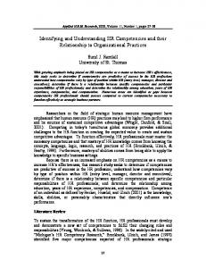
2.3 Forest transition Forests transition theory assumes that, in the course of economic development, industrialization, and concurrent emigration from rural areas to urban centers, forest cover starts to increase after periods of decline in early development stages (RUDEL, 1998). The lowest point on the curve of forest cover changes over time is named forest transition (MATHER, 1992), figure 2.3. Figure 2.3: Forest transition

Forest increase

Forest cover 

Forest decrease

Forest transition

Time

Source: MATHER, 1992.

According to RUDEL et al. (2005), there are two pathways of forest transition: forest scarcity pathway (a scarcity of forest product and/or decline in the flow of services provided to societies by forest ecosystems prompted governments and land managers to establish effective afforestation programs) and economic development (RUDEL et al., 2005). According to the economic development pathway, the labor force is driven from agriculture to other economic sectors and from rural to urban areas because of economic expansion (LAMBIN and MEYFROIDT, 2010); large areas of land that are marginally suitable for agriculture are abandoned and left to forest regeneration (LAMBIN and MEYFROIDT, 2010; RUDEL et al., 2005). Often, the forest transition also goes in hand with a switch from the dominance of agricultural institutions to that of forestry institutions (GRAINGER, 2010).

Chapter 2 | 9

MEYFROIDT and LAMBIN (2010) showed three more pathways of forest transition. They are state forest policy, tree-based land use intensification and ecological quality of forest transition, and globalization (MEYFROIDT and LAMBIN, 2010). Globalization is a more modern version of the economic development pathway that occurs when a national economy becomes increasingly integrated into global markets for commodities, labor, capital, tourism and ideas (RUDEL, 2002 cited in LAMBIN and MEYFROIDT, 2010). State forest policy is a new national forest/land use policies aiming to modernize the economy of land use, integrate marginal social groups, promote tourism, or foreign investments, geopolitical interest in asserting control over remote territories via the creation of natural reserves, managed state forest; tree-based land use intensification is driven by innovations in farming systems rather than by forest conservation (MEYFROIDT and LAMBIN, 2010). Ecological quality of forest transition implies that forests can change their ecological quality in each of aforementioned pathways, because they (pathways) can be associated with varying impacts on the delivery of ecosystems goods and services and with forests with different ecological qualities; for example, a country that would have depleted its primary forests and replace them by tree crop plantations could appear to undergo a forest transition (LAMBIN and MEYFROIDT, 2010). In addition, MEYFROIDT and LAMBIN (2010) states that forest pathways are not independent and interact in several ways, and certain forest transition pathways are more likely to lead to forest transitions with high ecological quality than others (LAMBIN and MEYFROIDT, 2010). Forest transition is studied firstly in Europe (MATHER, 1992; MATHER and NEEDLE, 1998) and later in Asia and other tropical forest countries (MATHER, 2007; RUDEL, 2010; RUDEL et al., 2002). Researchers that studied forest transitions in tropical forest countries have tried to explain the factors that cause the return of forests. Agriculture expansion and wood exploitation in the uplands, driven by population growth and migration from lowlands, caused deforestation in Vietnam from the 1970s to 1980s; later periods of reforestation were accompanied by political and economic changes as a response to the economic stagnation of the country after the 1980s (MEYFROIDT and LAMBIN, 2010). Forest transitions occurrences were analyzed at various spatial scales. Studies characterized sub-regions within a country (FARLEY, 2007; XU et al., 2007), an entire country (BAE et al., 2012; MATHER et al., 1999), or several countries within a large geographical region (RUDEL et al., 2005). The empirical evidence shows that forest use and, consequently, forest cover changes differ from one region to another, between countries (REDO et al., 2012), and sub-regions of a country (RUDEL et al., 2005). Priority has been given to empirical studies for forest transition (GRAINGER, 2010; MATHER, 2007). In this regard, post-socialist countries are interesting to study because governments might have implemented new land use and forest policies after the collapse of socialism, which could affect the occurrences of forest transition, e.g., could cause a delay of forest transition. Empirical studies could give their contributions to show the particularities of forest transition at country, but also

10 | Theoretical background on forest cover and use

at sub-region and region level as needed and cited from the literature of forest transition. Studies of post-socialism countries could also reveal worthy findings of forest transition occurrences from the beginning of the socialism until today. Such studies could compare the governmental interventions and policies of land use in two periods i.e., between period of socialism and post-socialism and, investigate the effects of socialism and post-socialism governmental interventions on forest services. For example, there are empirical evidences that indicate that forests in postsocialist countries experienced excessive timber extraction and including illegal logging decreased forest cover after the collapse of socialism in many countries of Eastern Europe and the former Soviet Union; subsequent forest increase, mainly in later periods of the transition, was mostly due to the natural forest succession of forests on abandoned agricultural lands (TAFF et al., 2010). Also, forests in these countries have a high potential for carbon sequestration because of forest increase (KUEMMERLE et al., 2011), and therefore these empirical studies show a way to tackle the climate change that has nationally, regionally and globally a positive impact to climate regulation, but also to forest biodiversity.

2.4 Spatially explicit analyses of forest cover change Statistical analysis is an important tool for models of land-use change. Regression analysis, for example, helps to quantify the contribution of the individual forces that drive land-use change as demonstrated by RIETVELD and WAGTENDONK (2004) and VERBURG et al. (2004a) thus provides the information required to appropriately calibrate models of land-use change (KOOMEN and STILLWELL, 2006). Also, land use change models are tools for understanding and explaining the causes and consequences of land use dynamics; they facilitate the integration of both environmental and human variables (CHOWDHURY, 2006; GLP, 2005; MÜLLER and ZELLER, 2002; NELSON et al., 2004; SERNEELS and LAMBIN, 2001; VELDKAMP, 2004; VERBURG et al., 2004b). Spatially exploratory statistical analysis have been also used to uncover the underlying processes that determine forest cover and forest cover changes (GEIST and LAMBIN, 2002; IRWIN and GEOGHEGAN, 2001; MERTENS et al., 2001; MÜLLER and ZELLER, 2002). GEIST and LAMBIN (2002), identified driving forces and proximate causes of deforestation in tropical forests consisting, respectively, of demographic (e.g., population density, population distribution, migration), economic, technological, policy (e.g., mismanagement), cultural factors (e.g., public that is unconcerned about forests), other factors (e.g., war, forest fires), infrastructure extension (e.g., road, settlements), agricultural expansion and wood extraction (commercial, fuelwood, charcoal production), for more information on the interrelations of these selected driving factors and proximate causes (see GEIST and LAMBIN, 2002), Figure 2.4.

Chapter 2 | 11

Figure 2.4: Causes of forest decline

Proximate causes

Infrastructure extension: Transport Markets Settlements Public service Private company

Agricultural expansion: Permanent cultivation Shifting cultivation Cattle ranching Colonization

Wood extraction: Commercial Fuelwood Polewood Charcoal production

Demographic factors: Natural Increment Migration Population density Population distribution Life cycle features

Economic factors: Market growth Economic structures Urbanization and industrialization Special variables

Technological factors: Agro-technical change Applications in wood sector Agricultural production factors

Other factors: Pre-disposing environmental factors Biophysical drivers Social trigger events

Policy and institutional factors: Formal policies Policy climate Property rights

Cultural factors: Public attitudes, values and believes Individual and household behavior

Underlying causes

Source: GEIST and LAMBIN, 2002.

Models of land use change and of deforestation utilize variables that are biophysical e.g., elevation, slope, soil type, rainfall, socioeconomic e.g., demographic (CHOWDHURY, 2006; MÜLLER and ZELLER, 2002; NELSON and HELLERSTEIN, 1997), urban growth (LONG et al., 2007), and policy (AGRAWAL and CHHATRE, 2006; DEININGER and MINTEN, 2002; GEIST and LAMBIN, 2002; LAMBIN et al., 1999) e.g., accessibility variables (CHOWDHURY, 2006; MÜLLER and ZELLER, 2002), protected areas (DEININGER and MINTEN, 2002).

2.5 Determinants of forest cover change and processes "The importance of the related concepts of the centrality of location and the influence of neighbors parallels the centrality of constrained (by resource or budget) utility maximization concepts for economists" (NELSON, 2002). Agricultural markets are used "to illustrate the importance of location and its corresponding transport costs to a central market when determining production (land use choices) at various locations and the resulting land rent" (NELSON, 2002), namely the theory of agriculture location von Thünen, which has still influence on nowadays research on land use despite the theory was formulated in 1826 (MORAN and OSTROM, 2005). The vicinity

12 | Theoretical background on forest cover and use

of forests to markets, the presence of roads are all used as determinants that have an impact on deforestation (DEININGER and MINTEN, 2002; MERTENS et al., 2001; NELSON and HELLERSTEIN, 1997). "Distance and travel times to road and markets serve as a proxy for prices and transaction costs (DEININGER and MINTEN, 2002) and access to political centers" (MÜLLER, 2003) and "lower values of these variables might be associated with lower forest cover because of higher producer prices, lower input prices and lower transaction costs compared to remote locations" (MÜLLER, 2003). Higher lagged population is often cited as a major factor influencing deforestation (DEININGER and MINTEN, 2002; MÜLLER and ZELLER, 2002). Forests in protected areas are better-protected from the deforestation, which means that less deforestation occurs in protected areas forests (DEININGER and MINTEN, 2002; GEIST and LAMBIN, 2002). Deforestation is caused by logging activities in areas accessible by roads. The government of Albania planned to rehabilitate forest roads for legal logging but the intervention of government to improve the forest roads encouraged the collection of wood that was not legal (THE WORLD BANK, 2004; THE WORLD BANK, 2007a). The long-term forest resources assessment database of European Forest Institute (EFI) showed that fuel wood and industrial wood were mostly used during socialism (from 1953 until 1990) in Albania and the Former Yugoslavia (where Kosovo was part) (EUROPEAN FOREST INSTITUTE, 2009). From 1990 until 2005, the removals of forests are still in statistics as "industrial round wood removals and wood fuel removals" FAO (2010b), i.e., wood were extracted as industrial and fuel-wood in Albania. Also, the author got confirmation that fuel wood and industrial wood were still important in Albania during the data collection in 2008. After the collapse of socialism in Albania, charcoal production and grazing in forests have caused forest degradation (THE WORLD BANK, 2011) and own observations. Forest fires are usually set by local people mainly for the increasing the productivity of pasture (observed during my work experience in Albania). The number of forest fires increased from 342 in 1996 to 1,182 in 2007 in Albania (FAO, 2010b). Agriculture statistics of Kosovo showed that fuel wood is important in rural areas of Kosovo for heating (STATISTICAL OFFICE OF KOSOVO, 2008). In sum, deforestation may be caused by wood extraction for firewood by local people, industrial wood in Albania and Kosovo and charcoal production, and forest fires in Albania, Table 2.1.

Chapter 2 | 13

Table 2.1: Determinants of forest cover change processes based on the literature and knowledge on Albania and Kosovo Determinants of forest cover change

Process

Reference

Extraction of wood: for firewood for charcoal production for export Forest fires Cropland abandonment in Albania Forests regeneration in commune forests in Albania Mined-areas and Unexploded Objects of Kosovo war

Deforestation

(European Forest Institute, 2009; Müller and Sikor, 2006; Statistical Office of Kosovo, 2008), own observations

Forestation

(Machlis and Hanson, 2008; Müller and Munroe, 2008; Taff et al., 2010; The World Bank, 2002) own observations

Albania and Kosovo have experienced high outmigration of population from rural to urban areas as well as abroad (CALOGERO et al., 2006; UNITED NATIONS DEVELOPMENT PROGRAM OF KOSOVO, 2004), which could mean less pressure to forests and allow forests to regrow. The post-socialism reform of agriculture in 1992 was associated with the refuse of marginalized and non-high quality agricultural land in Albania (THE WORLD BANK, 2002). The decline of agricultural cultivation may potentially lead to the natural expansion of forests in Albania and therefore to the increase of forest cover (MÜLLER and MUNROE, 2008; TAFF et al., 2010). The new forestry reform started to be implemented in 1994 in the post-socialism Albania, where local people and government were allowed to manage forests (THE WORLD BANK, 2011). Years of establishment of communal forest administration are expected to be positively correlated with forest cover, because more forests may grow naturally since local people let forests regenerate (AGRAWAL and CHHATRE, 2006; THE WORLD BANK, 2004; THE WORLD BANK, 2011) as well as some villages planted trees to protect soil from the erosion (THE WORLD BANK, 2011). Therefore, natural regeneration of forests and afforestation in communal forests could lead to the increase of forest cover. Forests in surrounding and inside of some of protected areas have experienced intensive illegal logging leading to the decrease of forest cover (THE WORLD BANK, 2004), which indicates that new institution of forest management and environmental protection failed to protect forests in some of protected areas. The forests near Unexploited Objects and Mines (UXOM) sites could be abandoned because they might be still dangerous to use them, (e.g. MACHLIS and HANSON, 2008). The author observed land abandonment in previous mined areas of the conflict 1998-1999 in Kosovo in border with Albania (during my work experience in Kosovo).

14 | Theoretical background on forest cover and use

Hypotheses of determinants of forest cover (change) Literature shows that relationships between variables vary across space (spatial heterogeneity). For example, the relationships between variables of environment and vegetation (KUPFER and FARRIS, 2007), socioeconomic and vegetation (OGNEVA-HIMMELBERGER et al., 2009), accessibility to infrastructure and forests varied (DEININGER and MINTEN, 2002). In this study, relationships between forest cover change and population, the distance to nearest roads, to human settlement, to protected areas and to forest edge are assumed to vary from one area to another in the study area. The sign of these relationships is ambiguous, Table 2.2. Table 2.2: Hypotheses of determinants based on the literature of forests, land use change, climate change Model

Biophysical

Demographic

Determinants

Forest cover

Reference

Elevation

+

(Agrotec.SpA.Consortium, 2004; Deininger and Minten, 2002; Müller and Zeller, 2002)

Soil type

+

(Deininger and Minten, 2002)

Village centroid (X, Y)

+

(IPCC, 2001; Thuiller et al., 2005)

Ecological regions

+

(FAO, 2000)

Population, population density

ambiguous

(Deininger and Minten, 2002; Müller and Zeller, 2002)

Distance to nearest human settlements Distance to nearest city and commune center

Ambiguous

(Deininger and Minten, 2002; Müller and Zeller, 2002; The World Bank, 2004; The World Bank, 2007a)

Communal forests

+

(Agrawal and Chhatre, 2006)

Protected areas

+

Distance to nearest protected areas Distance to nearest UXOM Distance to nearest forest edge Accessibility of forests at the beginning of period

Ambiguous

Distance to nearest roads

Politicalinstitutional

(Deininger and Minten, 2002; Geist and Lambin, 2002)

–

(Machlis and Hanson, 2008)

Ambiguous

(Deininger and Minten, 2002; Müller and Zeller, 2002)

Chapter 2 | 15

Elevation and soil type are expected to be positively correlated to the forest occurrences; the higher the elevation, the higher the forest occurrences (DEININGER and MINTEN, 2002; MÜLLER and ZELLER, 2002). Certain types of forests, for example, beech grows naturally in certain soils, in higher elevation than oak forests (AGROTEC.SPA.CONSORTIUM, 2004). Hence, the variables capturing soil types are expected to be statistically significant for forest cover (changes) in some regions. But the direction of influence is unclear a priori, because the forest cover change data does not contain information on the composition of forest species that may have allowed anticipating the effect of soil types. The geographic location of villages, measured as the centroid coordinates of a village, serve as proxies for climatic conditions. Albania has a Mediterranean climate in the west and south and a more continental climate in the east and northeast. Therefore, villages further north (larger Y coordinates) and villages further east (larger X coordinates) tend to have a cooler (lower temperature) and a more humid climate (more rainfall) than villages further in the south (smaller Y) and the west (smaller X). Differences and changes in climate conditions affect forests. For instance hotter and drier climate (i.e., smaller X and Y of a village) will result in increased risk of forest fires that negatively affect forest (cover), the forest ecosystem productivity and lead to biodiversity loss (likely of forests of a village) (IPCC, 2001; THUILLER et al., 2005). Therefore, it is expected that villages in south of Albania could have more changes of forest cover (more deforested area) than those in northern Albania because of the increasing occurrences of forest fires caused by hotter climate (increasing temperature) and drier (fewer rainfall events) condition during the summer but also because of the changes of temperature and rainfalls caused by the climate change. Ecological zones are useful information to provide insights on the changes of forest resources based on the natural features of vegetation (sometimes a vegetation can cover more than one country area) at large-scale, region level (FAO, 2000). Forests in Albania and Kosovo are subtropical dry forests "dominated by evergreen oak species" and "temperate continental forest ecological zones" consisting of different deciduous broadleaved forests, which are represented by "oak, mixed oakhornbeam and mixed lime-oak forests" according to FAO (2000). Therefore, more broadleaved forests are expected to grow naturally in subtropical dry forests and temperate continental forest ecological zones. A human settlement (point data) represent a larger populated area (town, commune where market and institutions exist), or village (consisting of a number of households). The distance to nearest human settlements is an accessibility determinant of forests by populated areas. Forests are accessed for fuel-wood (mainly by local people) and industrial wood (by licensed companies) to sell them in the market, for protection, managing and controlling forests any illegal and legal activity in forests by institutions. The sign of the distance to nearest human settlements, distance to nearest commune and city center, distance to nearest forest edge, the accessibility to

16 | Theoretical background on forest cover and use

forests from the beginning of the period with forest cover (change) on forest cover change is ambiguous, because accessible remote high forests could be extracted near villages, but also far from them (high remote forests are old-growth forests located in high elevated and far from populated areas). Evidences shows that most of logging (either legal or illegal) activities happened in high remote forests (MÜLLER and SIKOR, 2006; THE WORLD BANK, 2004).

3 M ETHODOLOGY

This chapter describes the methodological approach that was used in the current study. Geographically weighted regression (GWR) is described in this chapter. GWR is used to uncover the local nonstationarity of the relationships between forest cover change and its determinants. The selection of GWR model is based on the minimization of the Corrected Akaike’s Information Criterion. The calculation of the variance of local coefficients and Monte Carlo test are used to set-up a hierarchy of determinants to map the spatially explicit coefficients of determinants that are statistically significant and explain most of local variations of forest cover change.

3.1 Geographically weighted regression (GWR) Spatial analysis is useful because it allows reduce large datasets to smaller amounts of more meaningful information suggest hypotheses or examine the presence of outliers through exploratory techniques; examine the role of randomness in generating observed spatial patterns; and test hypotheses about such patterns and modeling of the spatial processes (FOTHERINGHAM et al., 2000). Spatial analysis applications appear in economics, geography, the social sciences, archeology, epidemiology, geology, the health sciences (FOTHERINGHAM et al., 2000), as well as in urban and regional planning (YU, 2006), and ecology (KUPFER and FARRIS, 2007; MORAN and OSTROM, 2005; OSBORNE et al., 2007), poverty analysis (EPPRECHT et al., 2008). Spatial effects are spatial heterogeneity and spatial dependency. Differences of location across space is known as the spatial heterogeneity effect, and similarities of locations are known as the spatial dependency effect (ANSELIN, 1988, 2006). Identifying and understanding differences across space (rather than similarities) is one of the many reasons to use GWR (FOTHERINGHAM et al., 2002). In addition, local statistics measure spatial dependency through spatial autocorrelation or Moran’s I (ANSELIN, 1995; FOTHERINGHAM et al., 2002). GWR was developed as an exploratory technique for examining data for their accuracy and robustness and suggesting hypotheses to test (also termed as pre-modeling) as well as for post-modeling exploration to examine the model accuracy and robustness (e.g., the mapping of the residuals from a model) (FOTHERINGHAM et al., 2000). GWR has been used to study the spatial nonstationarity and scale-dependency in the relationships between species richness and environmental determinants for sub-Saharan endemic avifauna (FOODY, 2004). The impact of nonstationarity on model prediction of the distributions of wildlife in Spain, Great Britain was the focus of the study carried out by OSBORNE et al. (2007); they used GWR arguing that GWR (local method in which there are as many GWR coefficients values as observations) is complementary to

18 | Methodology

GLMs, OLS (global method in which OLS coefficients have one value for all observations) revealing details of habitat associations and the properties of data, which global methods miss (OSBORNE et al., 2007). The comparison of GWR and ordinary least squares (OLS) was made to predict patterns of Pinus ponderosa (pine tree) in Saguaro National Park, AZ, USA, using topography and fire history variables (KUPFER and FARRIS, 2007). The authors of this paper showed that local regression coefficients displayed significant local variation for four out of the five environmental variables and "GWR model consequently described the vegetationenvironment data significantly better…and reduced observed spatial autocorrelation of the model residuals" (KUPFER and FARRIS, 2007). GWR is also used to discover spatial variation in the relationship between socio-economic and green vegetation land cover in urban, suburban and rural areas (OGNEVA-HIMMELBERGER et al., 2009). The major finding of this paper is that GWR (not ordinary least squares technique), ought to be used for regional scale spatial analysis, because GWR can account for local effects and displays geographical variation in the strength of relationship (OGNEVA-HIMMELBERGER et al., 2009). Contrary to most conventional econometric methods, GWR allows to discover the local non-stationarity, which could be otherwise neglected when most conventional econometric methods are employed such as ordinary linear regression (OLS) (FOTHERINGHAM and BRUNSDON, 2004; FOTHERINGHAM et al., 2002; KAMAR et al., 2007; OGNEVA-HIMMELBERGER et al., 2009; YU, 2006). In contrast to global models (e.g., OLS), local statistical methods such as GWR allow derive spatially explicit coefficients and goodness-of-fit statistics that can be mapped (FOTHERINGHAM et al., 2000; FOTHERINGHAM et al., 2002). GWR has two major advantages to spatial expansion, spatially adaptive filtering, multilevel modeling, random coefficient models, and spatial regression models that also tend to study local variation. It (GWR) is based on the traditional regression framework and it incorporates local spatial relationships into the regression framework and uses decay function that "weights" more neighborhood observations that are closer to the regression point (i) than those further far from the regression point (FOTHERINGHAM et al., 2000). The weighted function or decay function bases on two regression kernel approaches: the fixed kernel and adaptive kernel. By default the kernel is a Gaussian function, Figure 3.1a.

Chapter 3 | 19

Figure 3.1: GWR spatial fixed and adaptive kernel

wij

a) distance decay function for a kernel

i

j

b) adaptive kernel Sparse observations

Dense observations

Note: wij the decay function. i the regression point observation. j the neighborhood observation. Observations close to the regression point of i receive a higher weight than observations more distant from the regression point i, e.g., j. Thus, the GWR measures the relationships inherent in the model around each location i.e., regression point i. Each neighborhood observation j is weighted by the distance from the regression point i (FOTHERINGHAM et al., 2002). Source: Adaptive from FOTHERINGHAM et al., 2002 and EPPRECHT, 2003.

The observation i is the regression point and j is a neighborhood observation. Each neighborhood observation (j) is weighted by its distance from the regression point (i) by a fixed bandwidths kernel in the fixed kernel approach (FOTHERINGHAM et al., 2002). The adaptive kernel is used when the data are not uniformly distributed shown in the Figure 3.1b following FOTHERINGHAM et al. (2002). Therefore, the distance from the regression point i to neighborhood observation j varies, because "kernel adapt themselves in size to variations in the data density… the kernels have larger bandwidths where the data are sparse, and smaller bandwidths where the data are dense" (FOTHERINGHAM et al., 2000; FOTHERINGHAM et al., 2002) Figure 3.1b.

20 | Methodology

Local spatial relationship is calculated by GWR for all observations in both fixed and adaptive kernel approaches. Furthermore, "the estimated local coefficients are a function of the bandwidth of the spatial kernel selected" (KUPFER and FARRIS, 2007) for the model or a function of the number of neighbors of the spatial kernel selected if the data are not uniformly dispersed. When bandwidth increases then the distance decay decreases, in this case GWR results are closer to that of the OLS regression solutions (KUPFER and FARRIS, 2007). The steeper the decay function the more local coefficients are depending on the observations that are closer to the regression point i (FOODY, 2004; KUPFER and FARRIS, 2007) for example decay function in the right is steeper than in the left of the Figure 3.1b. A Corrected Akaike’s Information Criterion (AICc) is used to compare global local models to test which model performs better and to study the local patterns of relationships e.g., Ponderosa pine basal area and aspect (KUPFER and FARRIS, 2007). The comparison of GWR and OLS, GWR and GLMs is used in studies to investigate patterns of relationship between specie-environment (KUPFER and FARRIS, 2007), distribution of wildlife (OSBORNE et al., 2007), regional analysis (KAMAR et al., 2007). These studies showed that information provided by OLS model was not sufficient because OLS model lacked the patterns of relationships. GWR was a very good technique to use because GWR model provided information on local patterns and GWR model performed better than OLS model. Model-fit for GWR are Corrected Akaike’s Information and R-square. According to KUPFER and FARRIS (2007), the model R-square is not meaningful metric for selecting the best models or for comparing the models of GWR and OLS because a model with many variables will have a very good fit to the data, but may have few degrees of freedom; the over-fitting of the data and low predictive ability comes as the result (JETZ, 2005 cited in KUPFER and FARRIS, 2007). Furthermore, the best model is the one with the lowest AICc value because the model with the lowest AICc "explains correctly the data" (KUPFER and FARRIS, 2007) and is "the best approximating models" of the reality (BURNHAM and ANDERSON, 2002). The minimization of the AIC is used also to calibrate a kernel (FOTHERINGHAM et al., 2002), which is another reason of using AICc as a model-fit measure in GWR studies (see e.g. BICKFORD and LAFFAN, 2006; KUPFER and FARRIS, 2007; OSBORNE et al., 2007). Two good comparable models have a difference of AICc values less than 3 (FOTHERINGHAM et al., 2002). Robustness relates to the presence of outliers in GWR likewise in ordinary regression (e.g., OLS). Outliers are removed from the data and models are then often compared with and without outliers, but in case of GWR, outliers are harder to be identified. This is because GWR "downweights some less extreme "near-outliers" because of the shape of the decay function", even if the outliers are excluded from the analysis (FOTHERINGHAM et al., 2002). In this study, I focused on the investigation of local variation between forest cover change and determinants using GWR, because this method (GWR) is frequently used for studies of spatial heterogeneity of vegetation. GWR was used to study temporally

Chapter 3 | 21

and spatially differences of forest cover change in two countries and made a comparison with OLS models based on the hypotheses of three models (of forest cover change). Local variation is questioned and tested in GWR applications i.e., whether it occurs by chance or not. Monte Carlo test is suggested and used commonly in GWR studies (FOODY, 2004; FOTHERINGHAM et al., 1998; FOTHERINGHAM et al., 2002; KUPFER and FARRIS, 2007). However, Monte Carlo test is very computer-intensive (KAMAR et al., 2007). A second approach to detect the spatial nonstationarity of relationships is "by comparing the range of values of the local coefficients between the lower and upper quartile with the range of values at ±1 standard deviations" of the global coefficients (CHARLTON et al., 2003) that are obtained by OLS for the same model as GWR. Decomposed local variations was used and further explained in the section 3.1.3. This investigates if local variation was explained by local coefficients estimated by GWR based on the similar work of KAMAR et al. (2007) and to find out the determinant explaining the observed changes of forest cover in the study area. 3.1.1 Models Information-theoretic method is used in natural sciences (e.g., ecology, biology, and statistics) to find a parsimonious model as the primary philosophy of statistical inference (BURNHAM and ANDERSON, 1998; BURNHAM and ANDERSON, 2002). Roots of theory are based on a formal relationship that Akaike found "between Boltzmann’s entropy and Kullback-Leibler information (dominant paradigms in information and coding theory) and maximum likelihood (the dominant paradigm in statistics). This finding makes it possible to combine estimation (point and interval estimation) and model selection under a single theoretical framework: optimization" (BURNHAM and ANDERSON, 2002). According to BURNHAM and ANDERSON (2002), "reasonable data and a good model" allow a separation of "information" from "noise". Here, "information relates to the structure of relationships, estimates of model parameters, and components of variance" (BURNHAM and ANDERSON, 2002). The principle of parsimony requires "a set of candidate models that involves professional judgment and representation of the scientific hypotheses into the model" (BURNHAM and ANDERSON, 2002). The principle of parsimony allows select the best fitted model based on the information criterion, which are Akaike Information Criterion, Corrected Akaike Information criterion and Akaike weights (BURNHAM and ANDERSON, 2002). Therefore, it is assumed that best model is sufficient for "making inferences from the data" (BURNHAM and ANDERSON, 2004). Hypotheses of three models are set a priory describing on plausible driving factors of the processes of forest cover change based on an extensive literature review of land use change, of deforestation, of land use and forests for Albania (as well as I refer to data of the European Forest Institute (EFI), own work experiences in forestry in my homeland and data collection in the study area in 2008). Data used for the current study were set into three separate models consisting of biophysical, demographic

22 | Methodology

and policy determinants. In this study, biophysical determinants were elevation, soil type, ecological zones, village locations. Demographic determinants consisted of population. Policy determinants composed of political and institutional determinants that were protected areas, years of establishment of Albanian communal forest administration, distance and cost distance for Albania and distance variables and protected areas for Kosovo. The scope of the current work is to find the determinants that explain the changes of forest cover and therefore the causes of the decrease and increase of forests. Biophysical determinants were thought to be surrogate of natural growth of forests assuming forests were extracted by people because of their abundance, naturally old-growth mostly as firewood for heating and industrial wood for profits (JANSEN et al., 2006; MILLENIUM ASSESSMENT, 2005a; MÜLLER and SIKOR, 2006); socioeconomic model (demographic model), assumed that people used forests for firewood (EUROPEAN FOREST INSTITUTE, 2009) and grazing (own observations). Model of political-institutional determinants assumed that people utilized more accessible, abundant and naturally well-grown forests for fuel-wood (i.e., firewood and charcoal to sell), and for industrial-wood (legal and including illegal logging) for profits (MÜLLER and MUNROE, 2008; MÜLLER and SIKOR, 2006; THE WORLD BANK, 2004). Models of political and institutional determinants included policy variables consisting of the distance to nearest roads, distance to nearest human settlements and distance to nearest mined and contaminated sites of Kosovo war. Institutional determinants consisted of the new administrations established in the post-socialism, specifically, commune administration and the establishment of forest user associations, new forest administration concerned the management of forests in protected areas, and new environmental agencies concerned the protection of environment and biodiversity in protected areas and environmental protection in forests. The setting-up of new post-socialist institutions (of communal forests and protected areas) is interlinked to the change of political regime. Years of establishment of communal forest administration is an institutional variable, which also implies a political decision to give forests from central to local government and local people to manage forests. Protected areas entails the institution that are established to plan, design, establish and manage existing and new protected areas and it also implies the political decision for the planning, management and the expansion of protected areas. For this reason, policy and institutional variables are labeled politicalinstitutional model.

Chapter 3 | 23

3.1.2 GWR equations The GWR approach relaxes the assumption of the OLS approach (equation 1), namely, that the relationship between the response and determinants has to be spatially constant (FOTHERINGHAM and BRUNSDON, 2004; FOTHERINGHAM et al., 2000): p

y i   0    i xi   i k 1

(1)

where β0 is a constant, βi is the coefficient, x is the value of the independent variable and ε is the error, y is the dependent variable, i is the observation, p total number of observations, k is the index of observations. This is done by considering the spatial location of the sample points for fitting the regression coefficients (equation 2): p

y i   0 (u i , vi )    i (u i , vi ) xi   i k 1

(2)

where (ui, vi) reflects the spatial coordinates of the sample in space, and (ui, vi) represents the centroid of each village, β0 is a constant, βi is the (GWR) local coefficient, x is the value of the independent variable and ε is the error, y is the dependent variable, i is the observation, p total number of observations, k is the index of observations. This approach allows the consideration of spatially varying effects of determinants on forest cover change. GWR fits OLS models based on a subset of spatial proximate sample observations. This means that the regression coefficients are estimated for a specific location (ui, vi) based on a number of sample observations. The influence of each observation in the regression model is thereby dependent on its distance towards the regression point (i.e., i) to be estimated. In other words, a weighted least squares regression is performed, and the weights are based on the distance to the regression point i at which the response is to be estimated. This leads to parameter estimation equation 4, which is a slight modification of the related OLS parameter estimation equation 3: ˆ  ( X T X )  1 X T y

(3)

ˆi  ( X T Wi X ) 1 X T Wi y

(4)

where Wi is a weight matrix in which off-diagonal elements are set to zero (i.e. non-correlated errors), ˆ represents the vector of global parameters (eq. 3) to be estimated, ˆ i is the vector of local parameters (eq. 4), X is the matrix of independent variables with the elements of the first column set to 1 and y represents a vector of observations on the dependent variable (FOTHERINGHAM et al., 2000). The calculation of the weights is based on a kernel regression approach. The default Gaussian weight, which is used in the current study, for the adaptive kernel are calculated using equation 5 for different neighborhoods:

24 | Methodology

 d 1   ij wij    hi  0 

  

2

   

2

if d ij  hi if d ij  hi

(5)

where hi defines the bandwidth of the kernel for regression observation i, which depends on the number of nearest neighbors selected and dij is the distance between regression point (observation) i and neighborhood observation j. 3.1.3 Decomposition of local variation The variance of the expected impact of a coefficient is based on the effect of the spatially-varying determinant values, as well as on the spatially-varying coefficients. Since both effects might be correlated, this needs to be reflected in the equation (KAMAR et al., 2007) that was based on Kmeta’s equation (KMETA, 1986) (equation 6). For determinant k, the equation reads as follows:  z Var ( z k   k X k )   k  X k

2

  z  Var ( X k )   k    k

2

  z  Var (  k )  2Cov(  k , X k ) k   X k

 z k    k

  

(6)

where β is the local coefficient, x is the value of independent variable, z is the β multiplied by x. Since both variables are known in zk, calculating the partials simplifies as follows: the first partial equals the mean of the squared βk (or local coefficients obtained by GWR) values, the second partial equals the mean of the squared Xk values (or explanatory variable X values) and the third partial equals the product of the mean of βk and Xk values. A cut-off of 0.50 is defined for the values of the variance of local coefficients (KAMAR et al., 2007). This cut-off help distinguish considerable determinants (the value of variance of GWR coefficients above 0.50) from non-considerable determinants (the value of variance of GWR coefficients below 0.50). A determinant with a variance of the local coefficient above 0.60 is considered important, and a determinant with a variance of the local coefficient above 0.70 is considered highly important. 3.1.4 Principle components analysis (PCA) "The main purpose of PCA is to condense the information contained in a large number of original variables into a smaller set of new composite dimensions, with a minimum loss of information. It reduces the P original dimensions of data set, where each dimension is defined by one variable, into fewer new dimensions, where each new dimension is defined by a linear combination of the original P variables. These linear combinations are called principal component…Principal components analysis creates new composite variables (or components) out of the original variables that maximize the variation among sampling entities along their axes… principal components are weighted linear combinations of the original variables that represents gradients of maximum variation within the dataset" (MCGARIGAL et al., 2000). "Principal components analysis assumes that variables change linearly along underlying gradients" and to assess the linearity assumption of principal components

Chapter 3 | 25

by graphing principal components that show "maximum amount of variation possible in a single dimension" to another the "second principal component that is constrained by orthogonality and maximization of the remaining variance" (MCGARIGAL et al., 2000). For example, if one has five principal components in an analysis where two principal components display most of variation, which let say component one and two then one makes a graph of the principal component one versus principal component two and see how the graph looks like. The linearity assumption is difficult for many relationships because the relationship can be nonlinear e.g., it is "particularly troublesome when attempting to ordinate species in environmental space" because the relationship between "frequency distribution of specie" show a Gaussian relationship (i.e., nonlinear) with an environmental gradient; in such a case "detrended correspondence analysis" is used to explain nonlinear relationships (MCGARIGAL et al., 2000) not PCA. 3.1.5 Generalized least squares (GLS) The spatial relationships of observations are nonlinear in GWR, because observation nearer a regression point i are weighted more than those far from it (i.e., regression point) (see section 3.1). Generalized least square (GLS) is used to proof that spatial relationships of observations are non-linear in the data of this study used. GLS is also used to study the heterogeneity of the relationships of the response variable and determinants, and identify the most significant determinants for the relationships (ZUUR et al., 2009). Firstly, the assumption of homogeneity is tested, by running a linear regression model, plotting the residuals using the restricted maximum likelihood estimation (REML) (ZUUR et al., 2009). Null hypothesis is the homogeneity exists between forest cover change and determinants. If residuals are not normally distributed with a mean of zero and a variance of σ2 (in a graph), then null hypothesis is not true. The GLS analysis is used to study the spatial heterogeneity (ZUUR et al., 2009). In this GLS analysis, four variance structure functions are used consisting of fixed, power, exponential, constant plus power of the variance covariate following ZUUR et al. (2009). "A GLS without weights is the same model as a linear regression model" (ZUUR et al., 2009). GLS is run once with weights and once without weights to compare the Akaike’s Information Criterion (AIC) values of GLS models to check which model performs better. "A fixed variance structure allows for larger residuals spread" if the distance to nearest human settlement increases (eq.7) var( ij )   2 x distance to nearest human settlements i

(7)

where sigma (σ) is the residual standard error, var (εij) is the variance structure, distance to nearest human settlement is a determinant. Weights of the power variance structure are specified as in equation 8: var( ij )   2 x distance to nearest human settlementsij

2

(8)

26 | Methodology

"The variance of residuals is modeled as  2 , multiplied with the power of the absolute value of the variance covariate" (ZUUR et al., 2009) i.e., of the distance to nearest human settlement. The parameter δ is firstly calculated. If the value of the variance of distance to nearest human settlements is zero, then, the exponential variance structure is used instead and not the power variance structure (ZUUR et al., 2009). The exponential variance structure is as in equation 9: var( ij )   2 x exp2 x distance to nearest human settlementsi 

(9)

The exponential variance structure models the variance of the residuals as  2 multiplied by the exponential function of the variance covariate of the distance to nearest human settlements) and the parameter δ is still to be calculated. In this case, "this structure allows a decrease of spread of values" of the distance to nearest human settlements in the case of a negative value of δi (ZUUR et al., 2009). The fourth model is the constant plus power of the variance covariant function, equation 10:



var(  ij )   2 x  1  distance to nearest human settlement s ij

2



2

(10)

"If δ1 and δ2 are zero" then one has a linear regression model, "if not then the variance is proportional to a constant plus the power of the variance covariance" (i.e., of distance to nearest human settlements) (ZUUR et al., 2009). The final model and the variance structure is selected by minimizing the AIC (ZUUR et al., 2009). Determinants with the largest variance within nested models ("two models are nested if one model can be obtained from the other model by setting specific parameters equal to zero" (ZUUR et al., 2009)) are selected, with the best model that is run once more with the "REML" method ("to find the optimal residual variance structure") (ZUUR et al., 2009); coefficients and sigma (σ) or the residual standard error are calculated. The determinant with the largest variance is the determinant that has the highest coefficient value in absolute terms and is multiplied by sigma (σ) in square. The largest variance value is the highest product value of these two. In the case of two good comparable nested models, the product values for each determinant per nested best models are compared; the largest product value shows the largest variance determinant (ZUUR et al., 2009). The author uses likelihood test for a full model and a nested model using maximum likelihood (ML) (ZUUR et al., 2009), to find the best fixed component, and distinguish the significant variables from nonsignificant variables. The ANOVAs with the full and nested model (one determinant is dropped) is run to calculate the likelihood ratio and p-values of the models (ZUUR et al., 2009). If the p-value is statistically significant at p-value 0.70). GWR local coefficients were calculated using the adaptive kernel approach (because of non-uniformity of data) with the number of neighborhoods of 30, 60, 90, 150, and 350. Local patterns were more evident with the number of neighbors 30 and 60. The number of neighbors was selected approximately 1 % of observations in Albania and Kosovo datasets, and approximately 10 % of the observations for the Albania-Kosovo cross-border area; because the model fit values of the Corrected Akaike’s Information Criterion-AICc of GWR models tend to be lower with the number of neighbors 1 % (at country level) and 10 % (at cross-border level).

28 | Methodology

Figure 3.2: GWR analysis flowchart Time period

1988-2000 2000-2007

Yes

Pearson correlation

Models

Biophysical Political and institutional Demographic

Test for the origin of local variation & Understanding of selected spatial local patterns of coefficients

Remove correlated determinants

No

GLS OLS

GWR No. neigh. selection

GWR model selection

SAC OLS Moran‘s I of residuals

model selection AICc permutation test SAC GWR Moran‘s I of residuals

In favor of GWR?

AICc

Yes

No

Models comparisons

Global estimates

Source: Adapted from SVEN LAUTENBACH.

A spatial weights matrix was created, using a queen’s contiguity neighbor, first order for the spatial autocorrelation of residuals (SAC in Fig. 3.2), in Geoda095i to calculate the Moran’s I of residuals (MORAN, 1948) in GWR and OLS. A Leung test was calculated to show the improvements of GWR towards OLS per model. Monte Carlo test for the final models of GWR was used to test the spatial variation with the permutation of 99 for the aggregated dataset of Albania, the Kosovan dataset and the cross-border Albania-Kosovo datasets, and the permutation of 9 with the Albanian disaggregated dataset because the Monte Carlo test with the Albanian disaggregated dataset was very computer-intensive. However, to double check the results for Albanian disaggregated dataset, the author also used the second approach used in GWR software by CHARLTON et al. (2003). The model with the lowest value of AICc was selected as the final model. GWR with response variable and all determinants of selected biophysical, politicalinstitutional and demographic models was also run. The next phase was the analysis of generalized least squares (GLS) and principal components analysis (PCA) of the GWR’s final models. The fourth and final phase (of the GWR methodological approach) was the calculation of the decomposition of local variation that was the test for the origin of local variation of the relationships between determinants and the response variable of GWR’s selected models. A determinant showed a strong

Chapter 3 | 29

local influence variation when the Monte Carlo test was statistically significant at p-value < 0.05 or below, and the variance of local coefficients was at and above a cut-off level of 0.5 (the cut-off level of 0.5 was decided based on previous study of KAMAR et al. (2007)). A determinant that had statistically significant value of Monte Carlo test (p-value < 0.05) and the variance of local coefficients above 0.7 was selected as the determinant to explain the changes of forest cover. The final stage of the analysis was the mapping of GWR results. Spatial local patterns of relationships between the response variable and the selected determinants from the final model were mapped out and discussed. 3.1.7 Added value of this research The GWR technique is used to explore the relationships of dependent and independent variable at the village level and shows how the relationships vary across the villages. Spatial heterogeneity is investigated using fine resolution data of forest cover and three distinctive datasets. The first datasets are composed largely of disaggregated determinants for Albania and Kosovo. The second dataset is made of aggregated and more complex determinants i.e., cost distance determinants for Albania. The datasets of the cross-border study region of Albania-Kosovo are extracted from Albanian and Kosovan disaggregated determinant datasets. For the first time, the heterogeneity of the relationships between the forest cover change and determinants are studied in two different periods from 1988 to 2000 and from 2000 to 2007 at country and region levels for Albania and Kosovo. The selected model is found by using the concept of inference statistics of the parsimonious model (henceforth "final model") (see the section of models) and the decomposition of the local variation (of forest cover change and determinant relationship) to find determinants that explain the strong patterns of the changes of forest cover. Determinants that have high values of the variance of GWR coefficients are at the top of the hierarchy of determinants. Deductively, I focused my interpretation and discussion around the results of these determinants. The analysis of generalized least squares (GLS) identified most significant determinants that had the largest value of variance of the relationships at the country level. This study focused not simply to identify patterns of forest cover change, explore local variation, but also to identify determinants of forest cover change that exhibited the highest local variation, and focuses the discussion on these determinants. This study provides a clear and new workflow of a GWR application focusing on spatially and temporarily changes of forest cover change at country and regional level for two understudied post-socialist countries and a post-war country. This work can help identify future research on forests for the study area. The entire methodological approach used in this study is different from studies on forests and from GWR application (to my knowledge), can be replicated for forests worldwide.

30 | Methodology

Descriptive statistics of forest cover change The raster layers depicting elevation, slope, distance to nearest human settlements, distance to nearest roads, distance to nearest town and commune center, distance to nearest major roads, distance to nearest protected areas, distance to nearest asphalted roads is transformed into a set of new layers by applying a "reclassification" operation in ArcGIS. This involves recalculating the value of a given focal cell into five quintiles (0 %, 25 %, 50 %, 75 %, 100 %). The input raster layer of forest cover change from 1988 to 2000 (and forest cover change from 2000 to 2007) overlaid to new layers of these explanatory variables (elevation, slope, distance to nearest human settlements, distance to nearest roads, distance to nearest town and commune center, distance to nearest major roads, distance to nearest protected areas, distance to nearest asphalted roads) to calculate the percent of forest cover change to five quintiles using "cell statistics" in ArcGIS. This involved recalculating the value of a given cell based on the mean value of forest cover in five quintiles (ESRI, 2009). This allows the number of forest pixels (in a quintile) to be multiplied by the resolution of forest pixels of 28.5 m and divided by the total number of forest pixels (see section 4). The vector layers depicting soil type, protected areas, and ecological zones were intersected with forest raster layers using "Zonal histogram" operation in ArcGIS. This involved forest cells intersected soil vector data generating a histogram, which was an output table consisting of a number of forest pixels for each soil type. This operation (Zonal histogram) is applied to calculate the percentage of deforestation and forestation to years of establishment of commune administration.

3.2 Generalized linear models (GLMS) Models are fitted using the Generalized Linear Models (GLMs) with a logit-link and binomial error structure for Albania-Kosovo cross-border analysis and habitat suitability modeling. "GLM is an extension of classic linear regression models that allow the analysis of non-linear effects among variables and non-normal distribution of the independent variables" (MCCULLAGH and NELDER, 1989). The Kruskall-Wallis non-parametric test is used before the analysis of GLMs. Independent variables are selected if they show statistically significant values with the dependent variables (p < 0.05). The remaining explanatory variables are checked with a Pearson correlation test to exclude highly correlated variables (Pearson’s correlation value r > 0.70) from the GLMs analysis. The predictive accuracy of fitted models is assessed using two approaches. The first approach is a cross-validation to validate the accuracy of the results. The cross-validation is calculated for the selected models. Cross-validation is used to avoid the over-fitting in the model (FERNÁNDEZ et al., 2003; KANAGARAJ et al., 2011). The second approach is the explained deviance (D^2) and the area under a Receiver Operating Characteristic Curve (AUC). A high value of AUC (i.e. > 90%) is "outstanding prediction" of the pair of presenceabsence (HOSMER and LEMESHOW, 2000). The spatial autocorrelation of dependent

Chapter 3 | 31

variable jeopardize the results (NAVES et al., 2003), for this reason spatial autocorrelation of the dependent variable was checked using Geoda095i. Spatial weights matrix was created, using a queen’s contiguity neighbor first order. 3.2.1 Habitat suitability modeling Endangered species present the "compositional diversity" for forest biodiversity (MILLENIUM ASSESSMENT, 2005b). The biodiversity in forests is very important element of global biological diversity, because biodiversity help sustain forest ecosystem functioning supporting other forest services (MILLENIUM ASSESSMENT, 2005b), e.g., recreation (see Chapter 2). Today, an extinction of a threatened species and or an endangered species is not only a loss of biodiversity at global-level, but also a decline of diversity (at different scale) in genetic, ecosystem and landscape (MILLENIUM ASSESSMENT, 2005b). Therefore, an extinction of endangered large carnivorous species is a straightforward loss of biodiversity in forests. Umbrella specie are at the top of the food web, and their presence is studied because they occupy areas of high biodiversity (RICKETTS et al., 1999). They also act as umbrella species for the "requirements of sympatric species" (BERGER, 1997), and can help locating and planning protected areas (CARO and O'DOHERTY, 1999). Brown bear, Eurasian lynx and wolf are three top-food web, forest-dependent and protected species in Europe (BREITENMOSER et al., 2005). Researches on umbrella species are made to specify breeding habitat (FERNÁNDEZ et al., 2003), habitat quality (FALCUCCI et al., 2009), habitat differentiation (MAY et al., 2008), habitat conservation (NIELSEN et al., 2006), the risk of species extinction (NAVES et al., 2003; WIEGAND et al., 1998) and species reintroduction in fragmented or human landscapes (KRAMER-SCHADT et al., 2004; WIEGAND et al., 2004). This thesis identifies suitable habitats for the critically endangered species of Lynx lynx martinoi (henceforth, "the lynx"), protected species of Ursus arctos (brown bear) and Canis lupus lupus (wolf) in Albania. Lynx lynx martinoi is a subspecies of Eurasian Lynx at a high risk of extinction with a population at the threshold of approximately 100 individuals distributed in Albania, Macedonia, Montenegro and Kosovo; 75 % of the population is expected to be only in Albania and Macedonia (ARX et al., 2004; BREITENMOSER et al., 2008; LARGE CARNIVORES ON THE BALKAN, 2004). Nature conservation organizations such as International Union for Nature Conservation (IUCN), Coordinated Research Projects for the Conservation and Management of Carnivores in Switzerland (KORA), and European Nature Heritage Fund (EURONATUR) are involved in conserving its habitat and maintainning its population (BREITENMOSER-WÜRSTEN and BREITENMOSER, 2001; BREITENMOSER et al., 2008; BREITENMOSER et al., 2005; LARGE CARNIVORES ON THE BALKAN, 2004). Forest and landscape degradation, illegal killings and low prey populations are some crucial factors that threaten the lynx (BREITENMOSER-WÜRSTEN and BREITENMOSER, 2001; BREITENMOSER et al., 2008; BREITENMOSER et al., 2005; LARGE CARNIVORES ON THE BALKAN, 2004). Landscape change activities and degradation are noted by specie experts as a genuine issue in Albania (BREITENMOSER et al., 2008).

32 | Methodology

Single specie ecological modeling at multiple scales is a natural-human habitat model that helps classify habitat quality and core areas of high conservation values such as brown bear in Spain, where natural models determine nutritional conditions and reproductive rate, and human models define carnivore mortality due to human disturbances (NAVES et al., 2003; NIELSEN et al., 2006). Further this study employs fine-scale geographical data and breaks up natural models into landscape, prey, refuge, and prey and refuge sub-models to understand whether prey, refuge, or both, or fine-scale heterogeneous landscape determines specie presence, as is the case of the endangered Iberian Lynx in Spain (FERNÁNDEZ et al., 2006; FERNÁNDEZ et al., 2003). A set of a priori hypotheses on habitat selection of species are identified describing different natural conditions and resources required for refuge, food and breeding of these species based on the ecology and biology that exists for the lynx and Eurasian lynx, brown bear and wolf. For example, these three species need elevated topography, stable, undisturbed, well-connected broadleaved, evergreen and mixed forests as a refuge and to breed and to search for food (NAVES et al., 2003), Table 3.1. Table 3.1: Hypothesis based on the literature for lynx, bear and wolf and their biology knowledge Model hypothesis Landscape

Refuge and food

Human disturbance

Natural

Description Three species require dense, high, stable and undisturbed forests and high elevation to refuge, breed and search for food Brown bear rely on oak and beech forests for food, in course waters for fish as well as and lynx on bare rocks for breeding Three species stay away from human settlement, roads, and areas with loss of forest cover, because they cause higher mortality, higher disturbance and lower habitat quality for breeding, refuge and food Three species need areas of forests and land that provide suitable habitats for refuge, breed and food; it combines the landscape, refuge and food hypothesis

Reference (Fernández et al., 2006; May et al., 2008; Naves et al., 2003; Wiegand et al., 2008) (Balkan Lynx Strategy Group, 2008; Fernández et al., 2003) (Kramer-Schadt et al., 2005; Naves et al., 2003)

Natural and human variables are grouped with respect to these hypotheses. These species stay away from roads, villages, urban areas, highly disturbed forested land (e.g., from logging), because of lower quality of habitat (KRAMER-SCHADT et al., 2005). Thus, variables are split into two categories, which are labeled "natural" and "human". Natural variables are thought to be surrogates for "reproduction and

Chapter 3 | 33

survival" of these species and human factors are thought to affect mortality of species, following NAVES et al. (2003). Natural factors are further divided into categories of "landscape", "refuge", "food", "refuge and food" to further understand factors that explained the observed presences of these species. The landscape variables consist of forest cover, elevation and the terrain ruggedness index. Refuge and food consists of beech pure and mixed with coniferous forests, mixed broadleaved forests, coniferous forests, bare rocks and soil, oak forests, forest cover connectivity, forest and woodland cover and distance to nearest forest cover. The human variables include village density, distance to nearest asphalted road, distance to nearest well-kept road, distance to nearest seasonal road, distance to nearest dwelling road and distance to nearest village (Table A4.5). This study supports the draft-strategy for lynx conservation in Albania and the FYR of Macedonia (BALKAN LYNX STRATEGY GROUP, 2008), providing needed scientific information on the home-range of the lynx. For example, previous studies in 1980s state that lynx have an average home-range of 38 km2 (BOJOVIČ, 1978). These are probably underestimated figures. Nowadays, the lynx monitoring in the FYR of Macedonia indicates a home-range of 100 km2 (BALKAN LYNX STRATEGY GROUP, 2008). This analysis attempts also to provide additional scientific information on factors that determinate the species presence considering effects of forest cover changes on species distribution in Albania. 3.2.2 Flowchart of the habitat suitability modeling analysis The distribution of Emerald species by bio-geographical regions as well as distribution maps for selected fauna species were made between 2005 and 2006 (COUNCIL OF EUROPE AND MINISTRY OF ENVIRONMENT FORESTS AND WATER ADMINSITRATION, 2006). Methods used by biologists to collect data consisting of the survey of lynx track on soft ground, snow and faeces, and the interviewing of local people as shepherds, hunters and foresters (BEGO, 2001). Photographs of the tracks and faeces were taken, and GPS (Global Position System) was used to collect the coordinates of presences of lynx and Emerald species (BEGO, 2000). Presence locations of the lynx in Albania 2001 were provided by Lynx compendium (CATS, 2011). Lynx distribution in Albania in 2001 marked presences as constantly occupied area (considered as permanent presences in our study) and single observation confirmed (considered as temporal presences in our study). The occurrences into two groups are based on the permanent and temporal use of habitats by carnivores. Permanent and temporal presences are summed up as our main dependent variable. These presences are mostly encountered in forested and high elevation areas, and in total these occurrences are of 24 and 19 for lynx, 41 and 54 for brown bear, 93 and 89 for wolf in the permanent and temporal categories, respectively (Figure 3.3).

34 | Methodology

Figure 3.3: Presences of lynx, brown bear, wolf and forest cover in 2000 in Albania

Source: EMERALD project and Lynx compendium of CATS, 2011.

This study uses pseudo-absences that are chosen randomly using the Hawths Tools (an extension in GIS), and are the same number as the numbers of permanent and temporal presences per species. There are two conditions of pseudo-absences selection: 1. Only one location is selected within spatial resolution of 1 km2, 2- pseudoabsences are to be located in forest areas and preferably within specie-suitable habitats because generating pseudo-absences further away from the optimum established by presence data may increase over-prediction of the model (CHEFAOUI and LOBO, 2008; KANAGARAJ et al., 2011). The spatial resolution of 1 km2 (Fig. 3.4) is selected as the unit of analysis based on the previous studies on Eurasian lynx (KRAMER-SCHADT et al., 2005; MAY et al., 2008). The analysis is conducted at the resolution of 1 km × 1 km grid. All the variables are calculated using the extensions available in ArcGIS 9.3 (ESRI, Redlands, California USA). For a list of variables used in the analysis (see Table A4.5). The presences-pseudo-absences response variable is run with all variables for a given neighborhood scale that remained after variable reduction from combining the landscape, refuge and food, and the human variables ("global" model).

Chapter 3 | 35

Figure 3.4: Flowchart of habitat suitability modeling Species Grid 1x1 km

Balkan Lynx Brown Bear Wolf

Pearson correlation

Exploratory variables

Presences & absences SAC dependent variables Yes

No

Multiple scale Human model

Is the variable significant?

Yes

No

Remove the variable

Multiple scale Natural & subnatural models

2000 2007

2000 2007

Yes

AICc

Model selection

Habitat suitability Prediction maps

AUC

CV

D^2

The model of GLMs is selected from the complete set of candidate models for a given hypothesis using AICc. The uncertainty on this selection is measured by weighting AIC scores by the score of the best model (wi). Model in year 2000 is the basis year of the study that is approximately the midpoint of the period of study and compared with model in year 2007. The predictions of habitat-best models are mapped out and the potential core areas for habitat conservations are identified per specie (Figure 3.4). Neighborhood variables are included in the analysis. This is because the presence of a specie could be determined by the amount of forested and semi-natural areas within a neighborhood corresponding to the scale of a specie’s home-range, e.g., the Eurasian lynx female home-range (SCHADT et al., 2002 cited in KANAGARAJ et al., 2011). A species moves within their home-range to meet its needs for food, refuge and reproduction. The brown bear’s and wolf’s home-range is alike and larger than a lynx’s; therefore, the neighborhood variables are at larger scale for bear and wolf than lynx.

4 D ATA

Chapter 4 describes the data used in the analyses. The first section of the current chapter provides general information on the study area, Albania and Kosovo and the cross-border Albania and Kosovo. Section 4.2 shows the sources of fine-scale forest data. Sources of biophysical, demographic and political-institutional datadeterminants are in Section 4.3. Section 4.4 describes explanatory variables that are used for the habitat modeling.

4.1 Study area Albania is situated in the Mediterranean Sea basin, and has an area of 28,748 km2 and a population of 3.1 million (CENSUS, 2001). Altitude varies from 0 m to 2,751 m above sea level (Figure 4.1) with mostly Mediterranean and continental climate. Figure 4.1: Study area of Albania, Kosovo, the cross-border study region and the geographic position of the study area

Source: ELPA, MAFR, ESRI.

Albania has approximately 21,096 km of asphalt, well-kept and seasonal roads, 2,884 villages with a population mean of 591 inhabitants per village (SD=663.26). From 1989 to 2001, the rural population decreased by a village average of -91 inhabitants causing the depopulation of rural areas. Agricultural land is suitable in the

38 | Data

lowlands, which comprises 25 % of the country, while 75 % of the country is hilly and mountainous and marginally useful for productive agriculture (MINISTRY OF ENVIRONMENT FORESTS AND WATER ADMINSITRATION, 2006). Elevated areas in northern and eastern Albania have a very low level of arable land allocation per capita in rural areas (THE WORLD BANK, 2002), and have less accessibility to infrastructure compared to western Albania. The regions of Kukës, Dibër, Elbasan, Lezhë and Shkodër have high rates of poverty and are among the regions with the highest unemployment rate, as well as the highest rural population outmigration rate (MINISTRY OF ECONOMY TRADE AND ENERGY OF ALBANIA, 2007; THE WORLD BANK, 2002). The Korça and Vlora regions have a more diversified economy, sources of employment and higher remittances (THE WORLD BANK, 2002). Forests and woodland comprise approximately 27% of Albania’s land area (SUESS, 2010). Forests and pastureland were state-owned during socialism. In 2005, the forests consisted of public-owned forests (98 %) and private-owned forests (2 %) (FAO, 2010b). The change of forest ownership from the state to private and from the central government to local government started after the collapse of socialism. Commune forests entails commune to administer forests and villagers to use forests aiming the regeneration of forests. This forest reform started in in 1996 in Albania (THE WORLD BANK, 2011). In total, 364 villages have used forests and pastures from year 1996 to 2000. The network of protected areas is approximately 10 % of Albania’s total area in 2006. Albania has high forest biodiversity (FAO, 2005). Albania has five forest types: Mediterranean shrub, oak woodland, beech forests, Mediterranean fir and alpine zone (FAO and DIDA, 2003). Mediterranean shrub, found mainly in the southern mountainous region, consists primarily of evergreen shrubs (e.g., Quercus ilex, Q. coccifera, Arbutus unedo, and Myrtus communis), deciduous shrubs and Mediterranean trees. Broadleaved trees such as Beech (Fagus sylvatica) and Quercus spp. are common tree species in Albania. Fir (Abies alba) replaces beech forests in the southern part of the country. Mountain pine occurs above the beech and fir forests under conditions of harsh climate and poor soils, at elevations of 1,600 to 2,100 m in the north and from 1,700 to 2,300m in the south; the three main specie are Pinus leucodermis, Pinus peuce and Pinus heldreichii (FAO and DIDA, 2003). The multiple uses of oak and beech forests, and the deforestation caused by clearing land for agriculture, have caused their massive degradation, the reduction of biodiversity and severe soil erosion (FAO and DIDA, 2003; META, 1993). Illegal logging is common in high forests, which have high economic and ecology values. This was particularly true in the late-1990s onward, as industrial wood used for export and/or charcoal production, as well as grazing and fuel wood used for heating in rural areas, could have contributed to the increase of deforested areas in high forests.

Chapter 4 | 39

Kosovo is a landlocked country with an area of 10,917 km2 (Figure 4.1). Its population is estimated to be approximately 2 million (STATISTICAL OFFICE OF KOSOVO, 2007b); the last population census occurred in year 1981. Altitude varies from about 200 m to 2,656 m above sea level, and the climate is Mediterranean and continental. Kosovo has about 8,232 km of highway, first and secondary roads, and about 2,195 human settlements; there are 30 communes and 7 regions, where communes are administrative local government units (STATISTICAL OFFICE OF KOSOVO, 2007b). According to the Statistical Office of Kosovo, arable land comprises 53 % of Kosovo’s total area, forestland 41 %, water areas 1 %, and other areas 5 % (STATISTICAL OFFICE OF KOSOVO, 2007a). According to the Agricultural Household Survey 2006, 47.7 % of arable land plots were sized from 0.1 to 2 ha (STATISTICAL OFFICE OF KOSOVO, 2008). Migration is highest in Gjakovë, Gjilan, Mitrovicë and Prizren, while Prishtinë and Ferizaj have experienced a population increase (UNITED NATIONS DEVELOPMENT PROGRAM OF KOSOVO, 2004). The highest disparities between rural and urban areas exist in education, lifetime and income per head in Kosovo (THE WORLD BANK, 2007b; UNITED NATIONS DEVELOPMENT PROGRAM OF KOSOVO, 2004). According to the Agricultural Household Survey 2006, most households in Mitrovicë, Prishtinë, Ferizaj, Prizren and Gjilan (see Fig. 5.2 for names and locations of these communes) rely on forests for firewood (STATISTICAL OFFICE OF KOSOVO, 2008). In 2007, forest land comprised 40.3 % of Kosovo (SUESS, 2010). Broadleaved forests occupy about 93 % (oak, beech and mixed oak/beech forests), with conifers making up the remaining of 7 % total forested land. Ownership of forestlands are, approximately: 41 % public and 33 % private, and 26 % unknown based on the Forest Inventory 2003 (MINISTRY OF AGRICULTURE FORESTRY AND RURAL DEVELOPMENT OF KOSOVO, 2007; STATISTICAL OFFICE OF KOSOVO, 2008); 8.3 % of the total area is protected. National parks make up about 84 % of total protected areas, natural monuments 10 %, natural zones 2 %, and preserved landscapes 4 % (STATISTICAL OFFICE OF KOSOVO, 2007a). Kosovo experienced conflict from 19981999, which can be phased into the preparation of war in 1998, conflict in 1999, and a post-conflict period, all of which produced residual unexploded ordnance (UXO), potential chemical contamination, landscape cratering, vegetation removal, soil erosion and socioeconomic disruption (MACHLIS and HANSON, 2008). Mine clearing started immediately after the conflict and lasted for several years. The conflict led to high migration to neighboring countries such as Albania, Macedonia, Montenegro and Serbia (INTERNATIONAL CAMPAIGN TO BAN LANDMINES, 2000a; INTERNATIONAL CAMPAIGN TO BAN LANDMINES, 2000b), and also led to a reduction of agriculture production (OGDEN, 2000). The cross-border study region of Albania and Kosovo is defined by the border of Albania and Kosovo. This area is approximately of radii of 25 km from the border

40 | Data

to select villages of Albania and Kosovo. The entire cross-border study region is of 4,917.7 km2 (Figure 4.1) The Albanian part is 2,413.5 km2 and it includes the Region of Kukës. Kosovo part is 2,504.2 km2 and includes the Peja and Prizreni regions, and three urban areas of Pejë, Gjakovë and Prizren (Figure 4.1). The Albanian villages have a higher elevation (of 814 m above sea level), and are located at larger distance to road (mean distance to nearest road is of 802 m) and to protected areas (mean distance to nearest protected areas is 12,180 m) compared to Kosovan villages (mean elevation of 688m above sea level, the mean distance to nearest road is 587 m, the mean distance to nearest protected areas 10,108 m, respectively). Distance to nearest human settlement is comparable for villages in both country sub-regions (distance to nearest human settlement is of 1,247 m for Albania and of 1,101 m for Kosovo, all are mean values of determinants).

4.2 Forest cover change Forest data of resolution 28.5 m derived from Landsat TM and ETM+ satellite images for ~1988, 2000 and 2007 were processed in the Geomatics Lab at the Humboldt University of Berlin with an overall accuracy of 93% and a kappa indices agreement of 0.85, and were provided by STEFAN SUESS (2010). The forest class consisted of forest patches greater than 7 pixels of Landsat. This class was composed of deciduous forests, coniferous forests and shrubs (with a height of greater than 3 m) and covering above the 50 % of a Landsat pixel. The non-forest class consisted of all non-forest land cover (urban land, agriculture land, pastureland, waters) (SUESS, 2010), Table 4.1. Table 4.1: Description of land cover classes Class name

Description

Forest

(Semi-) natural terrestrial vegetation (broadleaved evergreen forest, broadleaved deciduous forest, coniferous forest and mixed forest), cultivated terrestrial (broadleaved arboriculture, fruit trees, orchards, groves, nurseries, vineyards) and shrub forest All others: built up areas, urban and industrial areas, artificial and natural perennial water bodies, aquatic vegetation, beaches, bare rocks/soils, sparse trees and shrubs; rock outcrops, (herbaceous) crops, vegetated urban areas, grassland

Non-forest

Source: SUESS, 2010.

The sources of images were Eurimage and the Global Land Cover Facility (GLCF) of the University of Maryland. The GLCF provided large blocks of orthorectied and geodetically accurate global land data sets of the National Aeronautics and Space Administration (NASA). These data had a geodetic inaccuracy less than 15 m (SUESS, 2010). A ground truth data were collected by SUESS (2010) in August and September 2008 in the study area for training and validation purpose measuring approximately 600 control points using the Global Positioning System (GPS) and

Chapter 4 | 41

photographing these spots. To validate the results of satellite images, SUESS (2010) used the Quickbird images of resolution of less than 3 m, and the Google Earth. Topographic maps of the scale of 1:50 000 of the University of California were partly geo-referenced for the land cover of Albania in 1980s (SUESS, 2010). He used the approach of Support Vector Machine (SVM) chain classification approach (KNORN et al., 2009) for the satellite images of 1988, 2000 and 2007. The SVMs represent a group of non-parametric algorithms (HUANG et al., 2002), and is considered as one of the most recent developments in the field of machine learning (JANZ et al., 2007). All images and vector layers were projected to UTM Zone 34 N, datum WGS84. The masks of the analysis are the country boundary of Albania and Kosovo. This allows the data within the country boundary to be processed (ESRI, 2011). The forest and non-forest pixels are reclassified as "1" and "0", respectively. The pixels (forests, non-forests) are intersected with the village boundaries to count the number of forest pixels for each village. The number of forest pixels is multiplied by the pixel resolution (28.5 m) and divided by 10,000 to give the forest cover in hectares for 1988, 2000 and 2007 (eq. 11). The forest cover 1988 is subtracted from the forest cover 2000 presenting the forest cover change from 1988 to 2000 in hectares (eq. 12). The forest cover 2000 is subtracted from the forest cover 2007 presenting the forest cover change from 2000 to 2007 in hectares (eq.13) (Figure 5.3). The same calculation is made for non-forest pixels (equation 14); the total number of pixels represents the land cover consisting of the sum of forest and non-forest pixels per village (equation 15). Calculations for forest cover of 1988, 2000 and 2007 in km2 (equation 16), forest cover in percentage (equation 17), are as follows: FCHA ij  NFP ijx 28.5 x 28.5  / 10 000

(11)

FCCHA 00 j  FCHA 00 j FCHA 88 j

(12)

FCCHA 07 j  FCHA 07 j FCHA 00 j

(13)

NFCKM

2

TLCKM

2

ij

 NNFP ij x 28.5 x 28.5  / 1 000 000

ij  NFPij  NNFPij

(14) (15)

FCKM 2 ij  NFPijx 28.5 x 28.5  / 1 000 000

(16)

FCPER ij  FCKM ij/TFCKM

(17)

2

2

ij

where i is the time step of forest data i=1988, 2000, 2007; j is the number of observations j=1…3055 for Albania or j=1…1298 for Kosovo. TLCKM2 is the total land cover in km2, FCKM2 is forest cover in square km, NFCKM2 is non-forest cover in square km, FCPER is forest cover in percentage, FCHA is the forest cover in hectares, FCCHA00 is the forest cover change in hectares from 1988 to 2000 and

42 | Data

FCCHA07 is the forest cover change in hectares from 2000 to 2007 (Appendix Table A4.1, A4.2, A4.3). The forest cover change had negative and positive values. The negative values of the forest cover change presents a change of land cover from forests to non-forests, a forest decrease (designated as "deforestation" process of the forest cover change) and the positive values of the forest cover change presents a change of land cover from non-forests to forests, a forest increase (designated as "forestation" process of the forest cover change in this study). Forestation consisted of afforestation, reforestation and the natural expansion of forests (FAO, 2000) in this study.

4.3 Determinants of forest cover change Determinants are secondary geographic data that were collected from 2008 to 2009. Geographic data are vector, shape files and raster data. Albanian data are projected in a Gauss – Kruger coordinate system, Kosovan geographic data are in coordinate system of WGS 1984 UTM Zone 34 N. Albanian geographic data are re-projected from Gauss-Kruger to the WGS 1984 UTM Zone 34 N coordinate system, because this is the working coordinate system for all data. Human settlement, roads, ecological regions and Digital Elevation Model (DEM) for Albania and for Kosovo are provided by the Environmental Legislation and Planning Albania (ELPA) and the Ministry of Agriculture, Forestry and Rural Development (MAFR). Protected areas are from the Institute for Nature Conservation, Albania, and the Kosovo Agency for Environmental Protection. Forest types and land use categories are taken from the Albania National Forest Inventory (ANFI) (AGROTEC.SPA.CONSORTIUM, 2004). Brown bear, wolf and Lutra lutra (European otter) presence data are from the Ministry of Environment, Forestry and Water Administration in Albania EMERALD project (COUNCIL OF EUROPE AND MINISTRY OF ENVIRONMENT FORESTS AND WATER ADMINSITRATION, 2006). Lynx compendium are from internet source (CATS, 2011). Population data of Kosovo are taken from the Kosovo Statistical Office (SOK) publications. Soil data are provided by the European Soil Database (PANAGOS et al., 2012), uranium and mined coordinates are from the United Nations Environmental Program (UNEP, 2001), International Campaign to Ban Landmines in Kosovo and Albania publications (INTERNATIONAL CAMPAIGN TO BAN LANDMINES, 2000a; INTERNATIONAL CAMPAIGN TO BAN LANDMINES, 2000b). Vector and raster data are all aggregated at village level using GIS software before starting GWR the analysis. The resolution of DEM is 25 m for Albania and 50 m for Kosovo. The output cells of determinants are 25 m for Albania and 50 m for Kosovo. As opposed to pixel, which is an abstract term, the village has a socioeconomic feature, because it presents a group of villagers that make decision on forests (use, protect, conserve forests) shaping forested landscape and defining forest patterns (see Chapter 2). This helps also identify area within which villagers alter their

Chapter 4 | 43

village landscape (CRAWFORD, 2002; RINDFUSS et al., 2003; WALSH et al., 1999 cited in EVANS et al., 2005). Technically, the GWR analysis is possible with village as unit of analysis. In case of pixel as analysis unit, the GWR analysis could have been very time and computer-resource demanding. Albania dataset has a total of 3,055 observations and Kosovan dataset has 1,298 observations. Albania’s cross-border dataset has 183 observations and Kosovo’s set has 286 observations (extracted from the Albanian and Kosovan datasets). There are two types of determinants: categorical and continuous. Protected areas, soil type, communal forests and ecological zones are categorical determinants generated from vector data. The distance to nearest roads, the distance to nearest human settlement, the distance to nearest forest edge, the distance to nearest UXOM, the distance to nearest protected areas is calculated as the straight line distance to the nearest road for each village (ESRI, 2011). The accessibility of forest at the beginning of the period (i.e., in 1988 for the first period and 2000 for the second period) is calculated by using the cost distance algorithm. "It is conceptually similar to the Euclidean allocation function, in which each cell is assigned to its nearest source cell" (ESRI, 2011). However, "near" is expressed "in terms of accumulated travel cost" (ESRI, 2011). Algorithms used for dataset preparation appear in Appendix A4.4 4.3.1 Biophysical determinants Elevation and slope are derived from DEM provided by ELPA and MAFR, respectively. Ecological regions are provided by ELPA for Albania, and are as follows: the Pindus Mountain Forests, Balkan Mixed Forests, Dinaric Mountains Mixed Forests and Illyrian Forests. Soil types provided by the European Soil Database for Albania are Eutric Regosol, Calcaric Regosol, Cambic Arenosol, Eutric Cambisol, Regosol and Cambisol. Ecological regions provided by ELPA for Kosovo are the Pindus Mountain Forests, Balkan Mixed Forests, and Dinaric Mountains Mixed Forests. Soil types provided by the European Soil Database are Dystric Planosol, Luvisol and Ranker for Kosovo (Appendix Table A4.1 and A4.2). Humic Cambisols, Chromic Luvisols, Eutric Cambisols, Eutric Regosols, and Haplic Phaeozems are soil types used for Albanian cross-border region. Soil types of Phaeozems, Luvisols, Renzinas and Rankers are aggregated and used for Kosovo cross-border region. Pindus Mountain Forests, Dinaric Mountain Mixed and Balkan Mixed Forest ecological zones are used for Albania and Kosovo cross-border region (Appendix A4.3). 4.3.2 Demographic determinants There were approximately 100 villages without population data in Albania. Population data is entered in these records by equally distributing the commune’s population (to its villages); this assumption is made to run the analysis with all observations.

44 | Data

The Kosovan population estimation from 1991 has an accuracy of 90 % at the village level (personal communication with the staff of the Statistical Office of Kosovo during the data collection in 2008). There are 1,446 human settlement records in the population estimation from 1991, and 1,298 observations (i.e., villages, town) from the cadastral data. Village names of the population estimation in 1991 were firstly translated from Serbian in Albanian. Names of villages in the population estimation in 1991 with the names of observations were carefully checked. Cadastral data were named after the human settlement names in 1991. The author assumed that the names of the human settlement boundaries would match the names of the villages in the population estimation from 1991. If the name of the observation matched the name of human settlements in the 1991 population estimation, the value of the population estimation in 1991 was manually entered to the respective village name in the dataset. In case of no match, "n. a." – no data was entered. The projected 2004 population at the commune level is used to obtain the 2004 population data at the village level. The projected 2004 village population is estimated as in equations 18 and 19. VPOP 1991  CPOP 1991 /NOV 1991

(18)

VPPOPj   CPPOPk/ k VEPOPj  xVEPOPj

(19)

where k is the number of communes k=1…30, j is the number of observations j=1…1298 for Kosovo. VPOP1991 is the population of villages of Kosovo in 1991; VPPOP is the projected population of villages of Kosovo in 2004. 4.3.3 Political-institutional determinants Human settlements include cities, suburban areas and villages. Roads consist of three types: main, major, and seasonal village roads in Albania. They are of three types in Kosovo: highway, first and secondary roads. There are six protected area categories according to IUCN (International Union for Nature Conservation) in Albania, and two in Kosovo. Protected areas are as follows: Strictly protected areas – category 1; National parks – category 2; Natural monuments – category 3; Nature resource management – category 4; Landscape protection – category 5; Managed Resource Protected Area – 6. There are two aggregated protected areas as follows: protected areas from categories 1-4 and protected areas from categories 5-6 (figure 7, 8). "Years of establishment of communal forest administration" is the number that shows the difference between the year the communal forest was established (e.g., 2000) and the initial year of the forest reform in 1996. Forests of 364 villages that were transferred from the central to the local communes from 1996 to 2000 are considered in the analysis. Forests of a total of 14 villages were transferred from central to local government in 1996, of 4 villages in 1997, of 18 villages in 1998, of 185 villages in 1999, and of 143 villages in 2000.

Chapter 4 | 45

Unexploded ordnance and mines (UXOM) include depleted uranium bombs and mines remaining from the 1998-1999 Kosovo Conflict. The coordinates of approximate bombed areas are geo-referenced (see UNEP, 2001). Mines (point data) are geo-referenced from the reports on mine clearance in cross-border AlbaniaKosovo and Kosovo-Macedonia (INTERNATIONAL CAMPAIGN TO BAN LANDMINES, 2000a; INTERNATIONAL CAMPAIGN TO BAN LANDMINES, 2000b) (Appendix Table A4.1, A4.2, A4.3)

4.4 Habitat suitability variables There are 24 permanent and 19 temporal presences of lynx, 41 permanent and 54 temporal presences of brown bear, and 93 permanent and 89 temporal presences of wolf. Lynx presences are geo-referenced from lynx compendium (CATS, 2011). Land use classes are grouped into eight categories: beech, oak, broadleaved deciduous forests, coniferous forests, cultivated areas, Mediterranean shrub areas, bare and rock areas, urban and industrial areas from (AGROTEC.SPA.CONSORTIUM, 2004). Lutra Lutra (European otter) presences are added as a biological indicator. Lutra Lutra relies on fish and its occurrences help to define (fish) food habitats of lynx and bear because they consume fish (BALKAN LYNX STRATEGY GROUP, 2008). A neighborhood variable was the mean value of the original variable within a specified neighborhood radius around the target cell of 1 km2 (moving window in GIS). In total, 5 different radii (3, 4, 5, 10 and 15 km) are used representing areas of 28.3 km², 50.2 km², 78.5 km², 314 km², and 706.5 km², respectively for the lynx and 7 radii (3, 4, 5, 10, 15, 20 and 25 km) representing areas of 28.3 km², 50.2 km², 78.5 km², 314 km², 706.5 km², 1256 km² and 1962.5 km², respectively for brown bear and wolf (Table A4.5).

5 R ESULTS

The patterns and processes of forest cover change are presented in section 5.1. The results of descriptive analysis are in section 5.2 and of GWR regression analysis in section 5.3. Differences between Albania and Kosovo at country level and subregion level and the synergies between GWR and GLMs are shown in this section. Discussion is focused on the results obtained by GWR that are patterns and processes of forest cover change. Results of the modeling of habitat suitability are shown in section 5.4.

5.1 Patterns and processes of forest cover change Albania shows more absolute changes of forest cover from the first to the second period compared to Kosovo. Deforestation dominates in the first period and forestation in the second period in both countries (Figure 5.1). Figure 5.1: Forest cover change in Albania and Kosovo

Note:

Forest data are provided by SUESS, 2010.

Source: Own calculation.

Three observations of forest cover in 1988, 2000 and 2007 show a slight increase of forest cover for Albania, the cross-border Albania and Kosovo (87,000, 88,000 and 90,000 hectares for Albanian cross-border part and 82,000, 84,000 and 88,000 hectares for Kosovan cross-border part for 1988, 2000 and 2007 respectively), and no increase of forest cover in Kosovo, Table 5.1. This conclusion bases on these time steps observations of forest cover (1988, 2000 and 2007). In fact more observations are needed to see how the trajectory of forest cover and forest transition

48 | Results

changes for each country, i.e., whether it goes up or down. In this regard, it is also worthy to have observations of forests after 2007, i.e., from 2008 until today (2012) to see if forest transition is occurring indeed or not in Albania and Kosovo. Observations of forests should be based on the same source that is the satellite-basedobservation and the same methodological approach of processing of forest data should be used, in order to have solid forest data over time. Table 5.1: Forest transition occurrence in Albania, the delay in Kosovo Year Forest cover change in ha (000)

Albania Kosovo

1988 767 445

2000 750 433

2007 805 433

Note: Forest data are provided by SUESS, 2010. Source: Own calculation.

Figure 5.2 shows forest cover changes using forest data of SUESS (2010), aggregated to the village level. Patterns of forest cover change alter from 1988-200 to 20002007. Deforestation (red color) is spread from the northern to southern Albania and northern and western Kosovo in the first period (1998-2000), while concentrated in the northern and eastern and western Albania and the northern and central and southern Kosovo in the second period (2000-2007). Figure 5.2: Forest cover change in Albania and Kosovo at village level

Source: Own calculation.

Chapter 5 | 49

Forest has increased (in green color) in the western Albania and eastern and southern Kosovo in the first period as well as in central and southern Albania and western and eastern Kosovo in the second period (Fig. 5.2).

5.2 Descriptive analysis of forest cover change 5.2.1 Albania Positive values of forest cover change in the determinant quintiles represent forestation and negative values deforestation. Forest cover change is in percentage to five quintiles of determinants. Forest of the first quintile is forest in low elevation; forest of the third quintile is forest in middle (range) elevation and forest of the fifth quintile is forest in high elevation, remote forest. For distance to nearest roads, forest of the first quintile is forest located near roads, of the third quintile is forest located in middle distance from road and forest of the fifth quintile is located at far distance from the roads. Forest of the fifth quintile of roads, human settlements is a remote (area) forest. In Albania, deforestation is stronger and more spread in higher elevations and long-distance accessibility areas or in remote areas (far from roads and/or human settlements). Forestation is higher in low elevations, and close to roads, and human settlements (Figure 5.3). Figure 5.3: Percent of forest cover change to five quintiles of determinants, Albania

50 | Results

\

Chapter 5 | 51

Source: Own calculation.

Forests close to protected areas and in protected landscape are cut as well as in strict protected areas (from 2000-2007). Forests tend to increase in large-distance from protected areas, and national parks (Fig. 5.3). Therefore, the remote areas (located in high elevation and far from human settlements) have experienced deforestation. Forestation and deforestation is present in commune forests. Deforestation has higher values from 1988-2000 compared to 2000-2007. The forestation process dominates from 1996-2000, while its values are higher from 2000-2007 than from 1988-2000. (Table A5.1: Forest cover change in commune forests). 5.2.2 Kosovo Deforestation is encountered in high elevations, far from human settlements, highway, protected areas, and UXOM sites. Deforestation is encountered in the first quintiles of the nearest distance to protected areas, and human settlements from 1988-2000. Forestation occurs in low elevations, close to human settlements, highway, protected areas, and UXOM from 2000 to 2007 (Figure 5.4).

52 | Results

Figure 5.4: Percent of forest cover change to five quintiles of determinants, Kosovo

Chapter 5 | 53

Source: Own calculation.

54 | Results

The highest value of deforestation is of -0.84 from 1988 to 2000 of the distance to nearest UXOM sites and of -0.83 from 2000 to 2007 of elevation. The highest value of forestation is observed in the low elevation (of 0.58 from 1988-2000, and 0.71 from 2000-2007, respectively) (Figure 5.4). 5.2.3 The cross-border study region of Albania-Kosovo Deforestation is estimated in all quintiles of variables in Albania and mostly in the fourth and fifth quintiles in Kosovo (Fig. 5.5). Forestation is observed mostly in the first and second quintiles of variables in Albania, and in the first, second and third quintiles of variables in Kosovo. In Albania, deforestation takes place in the middle and high elevations, in steep slopes, far from protected areas, far from the populated areas and UXOM of Albania. Deforestation is observed in high elevations, steep slopes, and areas that are hardly accessible from roads, close to protected areas, large distance human settlements, and UXOM sites in Kosovo in both periods. Forestation occurs mostly in low elevations, gentle slopes, and areas accessible from roads, close to UXOM and in middle distance from protected areas, and human settlements from 2000 to 2007 in both countries (Figure 5.5). Figure 5.5: Percent of forest cover change to five quintiles of determinants, the cross-border study region Albania

Chapter 5 | 55

56 | Results

Kosovo

Chapter 5 | 57

58 | Results

Source: Own calculation.

Comparison between Albania and Kosovo. Forestation is mostly observed in low elevations, close to human settlements, and easily accessible areas in Albania and Kosovo from 1988-2007. Deforestation occurs close to protected areas in Albania (Fig. 5.3), but not in Kosovo from 2000-2007 (Fig. 5.4). In addition, calculation of forest cover in the protected areas shows that forest loss occurs inside protected areas (Fig. 5.3). Forest cover change generally has a higher value, either positive or negative, in Albania compared to Kosovo (Figure 5.5). Forest cover change processes (deforestation, forestation) appear almost in all quintiles of determinants in Albania (Figure 5.3 and Figure 5.5) while deforestation is mostly concentrated in remote areas and forestation in accessible areas in Kosovo (Figure 5.4 and Figure 5.5). Despite forestation dominating in the second period, deforestation is present in both countries. 5.2.4 Interpretation and discussion of descriptive analysis of forest cover change Forest loss occurs within protected areas and close to protected areas (Figure 5.3., 5.4., 5.5) showing that high pressure exists on protected forests despite their status

Chapter 5 | 59

of protection. The protection of forests within protected areas is a responsibility of forestry, environmental protection and nature conservation institutions. Deforestation within these protected areas show that new institutions are unable to monitor forest activities in protected areas, tackle deforestation activities within them and control pressure inside and in the surrounding areas of protected areas. This supports the author’s assumption and literature on forests that protected area could ensure better protection for forests, but cannot guarantee a full protection and halt entirely the deforestation within them (DEININGER and MINTEN, 2002). Interestingly, forests close to mined areas have not been used by people as expected from 1988-2000. People began to use these forests (forests close to UXOM areas), from 2000-2007, when they were cleared from mines and became safer. In the case of Albania cross-border, it is different. Forests were used before the conflict of Kosovo (1998-1999). After the conflict (from 2000 to 2007 in this study), forests were used in far-distance from mined areas (Fig. 5.5). Deforestation occurs in almost all quintiles of the accessibility determinants of distance to nearest roads and human settlements in Albania compared to Kosovo at country and cross-border study region level. This shows that forests accessed by roads and human settlements tend to be used more in Albania compared to Kosovo. Roads make forests accessible for use. Forests at measured distance from human settlements are used regardless of the presence of an institution in commune, municipalities (human settlement). Observation and descriptive analysis of forest cover change (Figure 5.1 and Figure 5.3, 5.5) show that forests are reduced particularly in the first period, which indicates that firewood collection and logging have been intensive and new institutions have not been able to halt the spread of forest cutting activities. Forests in large-distance from human settlements are reduced. Deforestation has happened in the fourth and fifth quintiles of the distance to nearest human settlement in Kosovo and Albania at the country and cross-border study region level. In the second period, forest loss is encountered in the highest quintiles of the distance to nearest human settlement and elevation, indicating that forests in high elevations and remote areas are utilized for firewood and industrial wood. The distance to nearest road and human settlement are very much associated with deforestation at high quintiles in Kosovo, which shows that firewood collection is still important for remote areas, as indicated by STATISTICAL OFFICE OF KOSOVO (2008). Forest has generally increased in low elevations, close to human settlements in Albania and Kosovo from 1988-2000 and from 2000-2007. Potentially, forests close to roads and human settlements are less used because people tend to use forests in higher elevation that are more abundant and well-growth. Forests nearby the protected areas were used from 1988 to 2000 in Kosovo and Albania showing the high pressure to forests in surrounding areas of protected forests in this period. These forests located in surrounding areas of protected areas increased in Kosovo, but not in Albania and in the cross-border study region of Albania and Kosovo from

60 | Results

2000-2007. Forest has increased in commune forests for every year of establishment of the commune administration, showing that forest reform contributes, overall, to forestation (Fig. 5.3). However, there is an uncertainty if forests continue to increase overtime and if these forests and woodlands are used sustainably in all communes.

5.3 GWR modeling results 5.3.1 Albania The global correlation is high between the Pindus Mountain Forests and Illyrian Forests ecological zones (> 0.70). The Pindus Mountain Forest ecological zone is selected because the largest part of forests grown in this ecological zone. The final model consists of "political-institutional" determinants of GWR for forest cover change from 1988 to 2000 and from 2000 to 2007, based on the lowest AICc (Corrected Akaike’s Information Criterion) and contains fourteen determinants of Euclidean distances, protected areas and years of establishment of communal forest administration, Table 5.2. Table 5.2: Comparison between OLS and GWR models with disaggregated variables, Albania Model AICc AICc Moran’s I of the residuals 1988-2000 OLS GWR OLS GWR Biophysical 34298 33320 0.38 0.18 Biophysical including climate 34285 33209 0.38 0.15 determinants Demographic 34566 33926 0.44 0.26 Political-institutional 34462 33176 0.48 0.14 2000-2007 OLS GWR OLS GWR Biophysical 33121 31886 0.48 0.20 Biophysical including climate 33046 31748 0.46 0.15 determinants Demographic 33259 32250 0.50 0.26 Political-institutional 33178 31650 0.48 0.13 Note: Model selection estimator: Corrected Akaike Information (AICc), Moran’ I of the residuals. Source: Own calculation.

Values of R2 of the final model of political-institutional determinants range up to 0.80 for the first period and 0.72 for the second period, indicating the presence of the high local variation of the political-institutional determinants and forest cover change in both periods. Maps of R2 are displayed in the appendix Figure A5.3. GWR model models perform better than OLS because GWR models have a lower value of AICc and lower Moran’s I of the residuals compared to OLS, Table 5.1. The final models of political-institutional determinants, Table 5.2, explain forest cover change in Albania from 1988-2007 and from 2000 to 2007. The GWR models perform better than OLS model showing that patterns of the relationship exist

Chapter 5 | 61

between forest cover change and political-institutional determinants. The estimations of the decomposition of local variation and Monte Carlo test for fourteen determinants of the final models of 1988-2000 and nine determinants of final models of 2000-2007, respectively, show statistically significant values of Monte Carlo test (p-value < 0.01), the variance of local coefficients indicating the presence of the spatial variation in the relationships between forest cover change and GWR coefficients (Table 5.3). Table 5.3: Results of GWR models, Monte Carlo test p-value and the variance of local coefficients, Albania 1988-2000 Model

2000-2007

Variance of local coefficient

Monte Carlo test p-value

Variance of local coefficient

Monte Carlo test p-value

Elevation Pindus Mountain Forests Balkan Mixed Forests Cambisol soil type Regosol soil type Cambic Aerosols soil type

0.69 0.60 0.49 0.56 0.58 0.50

0.0 0.0 0.0 0.0 0.0 0.1

0.66 0.61 0.45 0.56 0.56 0.50

< 0.01 < 0.01 < 0.01 < 0.01 < 0.01 < 0.01

Population 2001 Population 1989

0.47

0.06

0.53

0.02

0.53

0.0

0.52

0.0

0.47 0.50 0.48 0.50

0.6 0.0 0.5 0.0

0.51

0.0

0.51

0.0

0.50

0.0

0.48

0.0

0.67 0.67

0.0 0.0

0.69 0.68

0.2 0.0

0.79

0.0

0.83

0.0

0.86

0.9

0.80

0.9

0.60

0.0

0.58

0.0

0.74

0.0

0.74

0.0

Determinant

Biophysical

Demographic Politicalinstitutional

Years of establishment of commune forest administration Strict Nature Reserve National parks Natural monuments Habitat or Species Management Area Protected Landscape or Seascape Managed Resource Protected Area Distance to nearest road Distance to nearest major road Distance to nearest asphalt road Distance to nearest human settlement Distance to nearest city and commune center Distance to nearest forest edge in the beginning of the period Distance to nearest protected areas

Note:

Levels of significance for Monte Carlo test p-value: