required. Many techniques have been used for image aata compression. / such as with ... t~rough DPCM and adaptive DPCM and at the end vector quantization.
IMAGE COMPRESSION USING BACKPROPAGATION NEURAL NETWORK DR.~
R M. ATTA,
S. EL FISHAWY, DR.M HADHOUD, PROF . K
H. AWADALLA
FACULTY OF ELECTRONIC ENG., MENOUF, EGYPT. 1. ABSTRACT Image data compression is a topic of increasing importance appears in situations where minimum
interest .
number
of
required. Many techniques have been used for image aata
Its ~s
bits
compression
/
such as with nonlinear t~rough
quanti~ation
and delta modulation, as well as
DPCM and adaptive DPCM and at the end vector quantization .
In this paper a three-layer neural network is used Backpropagation
the predictor of the DPCM.
to
algorithm
is
realize used
adapt the weights·of the network. The obtained results show performance (signal to noise ratio) specially for images
to
a
good
that
have
sharp edges and much details. Recorded imagesand computer simulation is used to verify the proposed technique. 2.Introduction Image compression is the problem of coding image data to reduce the amount of data that must be sent to 'transmit the image from location to another, where it. is reconstructed, over an
one
information
channel
(1).
Image compression is possible because nearby pixels
imag~s
are
often
highly
correlated .
which
allows
~hese
in
local
statistical relationships to be exploited . .Many techniques
reduce
transmission
rates
~y
reducing
the
redundancy or correlation within an image and then transmit this new set df d~ta. Predicti~e compression techniques operate the image pixels by use algorithms which make a currently
scanned
Subtracting the
based
pixel
predicted
reduces a difference, transmitted over the
or
value error
~hannel.
error sequence typically
upon from value
prediction
previously the
actual
which
directly
is
of
scanned
the
pixels.
scanned ~hen
on
value
coded
and
Data compression is achieved since the
has
II - 209
a
much
smaller
variance
than
the
.,
orig~nal
image
seq~ence
and thus require fewer bits
per
sample
in
its coded representation. One algorithm frequently
used
is
l2]
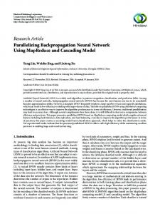
pulse code modulation ADPCM (Fig . 1) predic~ion
filter with
adaptive
the
adaptive
which
coefficients
differential
employs to
make
a
linear
the
pixel
prediction.
e(n,m) l(n,m)
-B---.-.
1 (n-m) Predictor .
f' (n,m)
~(n,m)
~(n,m)
PCM
I
J
·
(n-m)
Predictor
:
..................................................................... ............ .
Transmitter
Receiver
Fig.(!) Differential pulse code modulation system . In adaptive linear prediction, an adaptive capability such that the prediction filter coefficients
change
as
is the
used image
..
statistics change, producing a new filter more closely optimized to . the new set of image statistics . As a result, the error sequence will tend to maintain a low power. An algorithm which
has
linear prediction is the algorithm
provides
a
found
least simple
wide
mean
acceptance
square
LMS
computationally
adapting a set of linear prediction
for
adaptive
algorithm.
efficient
coefficients
to
This
way
of
nonstationary
data, and has been used successfully in several applications such as spectral
estimation
and
noise
cancellation
as
well
as
image
in
image
compression. Neural
networks
are
being
increasingly
used
processing, such as image recognition [3] and image restoration This
mainly
due
/
to
their
high
II - 210
computation
speed
and
[4]. their
' I
•
adaptability, which stems from learning capability.
In
section
predictoris
3
neural
presented~
network
model
and
its
Then, in section 4, computer
usage
as
a
simulation
and
results will .be given.
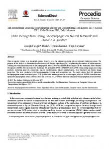
3 NEURAL NETWORK MODEL. By using three-layer feedtorward neural network shown in Fig with backpropagation algorithm to adapt the weig~ts of the we
~an
construct a predictor for the ADPCM.
network that has been successfully applied problems
ranging
compr,ession [ 5
from
to
a
wide
variety
image
to
scoring
of
J.
let the input preceded
network,
It is a powerful mapping
application
credit
2
pixels
of
the
·input·
first
P ( n, m-1) ,
P ( n, m-2) ,
P(n+l,m-2), P(n+l,m- 1), and P(n+l,m-2)
layer
be
the
P(h-l,m-1),
P ( n-1 , rn ) ,
to
the
currently
pixel P(n,m). Knowing the desired output of this pixel, we it from the actual output of the last 'output '
layer,
error only across the communication channel. At the error signal is used to reconstruct the
original
nearest
th~n
desired subtract send this
-· receiver,
pixel
adding.it to the output of its predictor and also is used
this
P(n,m)
by
to
adapt
network
(Fig .
the weights of its network.- · In. 2),
it~
simplest form · applying to the
the backpropagation training
three-laye~
~lgorithm
begins by
pr~senting
input pattern vector Xkto the network, sweeping forward through system to generate an output response of The output. Ykis in the form
Yk= I
/'
=
[k=O l wk
the
the error
[6] : (sk)
M where sk
Yk' and computing
N
I
[ j=O l
w. J
xj] ]
an
(i )
II-211 'I
•
and f
is a sigmoid logistic nonlinearity
1 f ( X)
= 1 + e
Where e is a threshold value . The output l a y e r
is in the
( 2)
- ( x - e)
error
of
each
the
in
element
fo~m :
( 3)
Where dk is the desired output of the network .
X
X X X
X
X X
1 2
3
_:)~ yk
4
5
,.
6
7
Fig . 2
.The next step
3-layer feedforward neural network
involves
sweeping
the
ef feet
of
the
backward through the network to associate .a square-error
errors
derivative
6 with each Adaline . The instantaneous square error derivatives first computed for each output layer. The
procedure
of
are
finding
6
hidden l~yer I involves 1 respectively multiplying each derivative 6(!- ) associated with each
associated
with
a
given
Adaline
in
element in the layer ' immediately downstream from a given Adaline the weight that connects it to the
given
Adaline .
These
weighted
square-error derivatives are then added together producing an term
e (I )
which,
· 1.n
t·urn ,
. l.S
. d mu 1 t.1.p 1 1.E!
by
sgm . ( s ( I ) ) ,
derivative of the g£ven Adaline is sigmoid function at operating point . Thus :
II - 212
its
by
error th e
current
•
•
(I )
1
=
0
( 4)
2
Each _n f _these derivatives in essence square output error of the network
tells is
to
output of the associated Adaline element. we use only one element in the output layer,
us
how
changes
sensitive in
the
linear
In the network used
layer
and
only
one
the
here, hidden
therefore we have only one 6.
6
The next step is to use this Adaline
gradients. Consider an during presentation k,
to
obtain
somewhere
in
the the
corresponding network
has a weight vector Wk' an input
and linear output sk= WT k Xk. The
instantaneous
which,
vector
gradient
·for
Xk, this
Adaline'element is
"' 2 (ck)
a vk
=
a
wk
"' 2 a (ck)
=
a
a a a
a a
sk "'
( £:
k
sk
a
sk "' 2 (ck)
a
=
a
)
,,
wk T
(XkWk)
wk
2 xk
sk
2 ok xk
( 5)
And finally updating the weights of each Adaline using the method of steepest descent with the
instantaneous
repe?ted by
ll-:Ll]
gradients. The
process
is
,
'
W = W + k+l k
= Where
n
factor, rate.
~(-V
k
Wk ... 2 i-1 6
ry(W k
)~
Xk
-t·
Wk_l) -
( ~J k -
i!
is the momentum constant, 0