Pruning backpropagation neural networks using modern stochastic optimization techniques Slawomir W. Stepniewski Department of Electrical Engineering (IETiME) Warsaw University of Technology ul. Koszykowa 75, 00-662 Warszawa, Poland
[email protected]
Andy J. Keane Department of Mechanical Engineering University of Southampton Highfield, Southampton, SO17 1BJ, U.K.
[email protected]
Abstract: Approaches combining genetic algorithms and neural networks have received a great deal of attention in recent years. As a result, much work has been reported in two major areas of neural network design: training and topology optimization. This paper focuses on the key issues associated with the problem of pruning a multi-layer perceptron using genetic algorithms and simulated annealing. The study presented considers a number of aspects associated with network training that may alter the behavior of a stochastic topology optimizer. Enhancements are discussed that can improve topology searches. Simulation results for the two mentioned stochastic optimization methods applied to nonlinear system identification are presented and compared with a simple random search. Keywords: optimization, neural network, pruning, genetic algorithm, simulated annealing.
1. INTRODUCTION
e.g., process age, oxygen consumption, carbon dioxide production, etc. Besides these basic plant models, other specially designed neural networks may operate as sensor/actuator failure detectors [20] or even function as direct controllers when a stable, inverse plant model exists [14].
Feedforward networks are perhaps the most commonly used among all types of neural networks. These networks seem to be an attractive tool for control engineering mainly due to the need for the flexible, accurate and inexpensive process models which they can provide. It should be emphasized that creating and validating alternative process models is sometimes a rather costly procedure. For example Bhat et al. [3] estimate that in the petroleum industry these costs can be as high as 75% of all the expenses associated with the development of a control system.
Obviously, in all these applications the maximal performance of the neural model is very desirable. The capabilities of control schemes generally improve as the synthesized model better matches the object. Well designed networks should also be as small as possible, especially for applications that require on-line model parameter adaption. Poor excitation or correlation between input signals and disturbances at the plant output, due to control feedback loops, commonly make identification conditions more difficult and oversized networks may then be prone to overfitting [13].
Neural models may be used in a number of ways in control systems. They may be employed as multi-step ahead predictors in optimal control systems [9, 14] or in transportation delay compensators (Smith predictors). One step-ahead neural predictors can be employed in reference model control schemes or related approaches [21, 14]. In some cases neural models function as Jacobian approximators of the controlled plant [2, 25]. Such Jacobians are required, for example, when the controller is also built using neural network techniques and needs to be trained while reflecting the influence of the plant. For these tasks neural models are especially useful when the nonlinear plant parameters vary in time or its analytical description is imprecise [2]. Neural models may also be used to estimate otherwise unavailable data for use by external controllers. Such problems occur, for instance, in technological processes that involve biomass fermentation [27]. In such cases, laboratory analyses introduce delays in sampling and are performed over such long intervals that they may cause operability problems for a given control system. Neural networks can then estimate unknown measurements based on more readily available outputs,
Finding a suitable neural network architecture for a particular application is still a challenging task. It is possible to experiment with hand crafted designs found by trial and error procedures but a much more appealing approach is to employ techniques that tune the network topology automatically. Methods developed for automated neural network topology design can be categorized into three major groups according to how they handle the problem of constructing network structures; a particular method can allow a topology to: - shrink only, - expand only, or - both shrink and expand. A series of methods that attempt to shrink or prune some given original architecture are described in [22]. For this 1
cost function used for topology optimization need not be the same as that used for the training phase. The proposed methodology allows great flexibility in setting up this function, since SA or GA do not make any assumptions about continuity or differentiability of the problem to be solved. In particular, they allow the user to introduce a variety of terms that quantify network complexity, generalization ability or network performance measured under conditions that emulate true working environments. Finally, the search may be conducted at various levels of detail, especially by a GA. It could be used not only for node or synapse removal but, for example, it could be extended to assign appropriate transfer functions for each node. A GA method can also be very easily distributed among several processors or computers as it operates on populations of solutions that may be evaluated concurrently.
task, one possible approach is to estimate the importance of each individual connection or whole node inside the network and then gradually to remove unnecessary components. A comparison of two such algorithms, Optimal Brain Damage (OBD) and skeletonization is covered for example in [8]. A more general approach than OBD is called Optimal Brain Surgeon (OBS) and is presented in [12]. Reduction in network size can be also combined with the process of network training. Weight decay and weight elimination approaches [13, 22] modify the learning law in such a way that it tends to lower the absolute values of connection weights so the weakest synapses can be removed if identified as being redundant. Probably the most well known example of a method that utilizes the expansion strategy is cascade correlation, designed by Falhman et al. [10]. This method progressively adds hidden nodes until the output error of the network decreases to a desired level. As a result a special kind of topology is created that may be viewed as a layered architecture with one node in each hidden layer connected to all previous nodes as well as the network input and output.
Besides these features, the GA and SA do not suffer from several of the shortcomings for which other pruning techniques are sometimes criticized. For example, sensitivity analysis based methods using second order expansion of the cost function are valid only if the weight changes are small [15]; as the synapse weight grows so does the error in its sensitivity estimation. Moreover, for some pruning methods, e.g. skeletonization or OBD, it has been observed that they tend to underestimate the importance of the elements that are located closer to network input [8]. These effects are especially problematic in 'wide' network architectures due to so called derivative dilution. In contrast to stochastic optimizers, OBD or OBS attempt to remove one link at a time. As was noted in [22] such techniques may not estimate correctly the importance of some configuration of connections such as where two weights cancel each other exactly. Removing either one leads to a significant error increase so their individual importance is then not negligible but in reality the whole pair is useless in performing the desired input-output mapping. Another difficulty with such methods is associated with the threshold definitions that are used to decide which network elements are important. This problem is especially severe in weight elimination or weight sharing schemes as it should not be assumed that small weight value is a reliable indication of redundancy.
Stochastic optimization techniques, such as genetic algorithms, have been employed for both network pruning and in the schemes that allow networks to grow and shrink. They use an objective function that reflects the overall performance of a network (complexity, accuracy, learning speed, etc.) to guide the search toward regions where promising architectures are more likely to be found. The methods often differ in the way they encode solutions and also sample the search space. A more comprehensive discussion of genetic algorithms applied to designing neural networks is carried out in the retrospective paper [18]. In this paper we focus attention on reducing the size of neural networks (without compromising network generalization ability or learning accuracy) using stochastic optimization techniques. We investigate the problem of pruning feedforward neural networks that are used to carry out nonlinear identification. The performance of two methods that have recently gained a great deal of attention - genetic algorithms (GA) and simulated annealing (SA) - are examined. These methods are additionally compared to a simple random search. As is shown later in this paper, such a comparison provides a rather severe benchmark for the methods under investigation.
The methodology presented here is similar to that described in [19] and [26], however, this study focuses on solving another, distinct class of problems. In the cited reports, topology optimization was tested on such tasks as the boolean XOR function, four-quadrant classification or the binary adder. On these tests, neural networks are expected to simply produce rapid changes in response for certain small deviations in their input. Therefore, such problems do not examine a very important feature of neural networks, i.e., their ability to generalize knowledge from examples. Good generalization means that a network is capable of producing smooth approximations of training data: four-quadrant classification or the logical XOR do the exact opposite. Of course, the different test problems investigated here require alternative, more appropriate methods to train the neural networks and to verify their performance.
Simulated annealing and genetic algorithm approaches provide several attractive features for developing near optimal network architectures. First of all, they offer a true separability between the stages of network training and architecture development. This allows hybrid systems to be designed for network pruning. Since the pruning procedures investigated here utilize only the overall, offline evaluated, network performance to guide the topology search, the same approach, as for feedforward networks, may be used for other network types, e.g., recurrent networks, that are better suited to function as multi-step ahead predictors, and which are typically more sensitive to architecture oversizing [4]. It is also worth noting that the 2
u( k )
NONLINEAR SYSTEM
y(k )
+
y$ ( k )
−
-1
z
-1
z
NEURAL NETWORK MODEL -1
z
e( k )
z-1
Figure 1: Modeling a nonlinear SISO system with a neural network (the scheme presented is off-line).
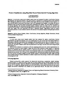
is also continuous. Figure 1 schematically illustrates the principle of modeling a nonlinear SISO system with a neural network.
As the problem becomes more complicated, so the size of the network and training data set increases and the training of a single network may become very slow. For this reason, most reported experiments in the field of combining genetic algorithms and neural networks have been tested on very simple examples. In some cases networks are not trained fully, instead their performance evaluated after some small number of cycles is used to estimate the final output error and the usefulness of a given design. This, however, may not reflect the true result when the network is allowed to train over enough epochs for convergence to be reached. To ensure more reliable estimates, the neural networks in our survey are trained fully at the expense of the greater time needed to complete the topology optimization. Also, we permit the optimization algorithm to sample a much bigger space of possible solutions by choosing relatively complex networks as the starting point for pruning.
A training algorithm adjusts the weights of the neural network to minimize a function Ψ defined as a sum of squares: N
Ψ=
N
1 1 L 1 L E L = ∑ ei 2 ( k ) = ∑ yi ( k ) − y$i ( k ) 2 2 i =1 2 i =1
2
(2)
where the parameter N L denotes the number of training patterns and e(k) is the difference between target and actual network output. The process of training is not, however, a pure, single objective optimization problem defined by a cost function Ψ. It is desirable that a trained network should not only produce a correct response for the training patterns but also for unseen data. Therefore, in the simplest case, to asses trained network generalization ability we may introduce another parameter, say EV , calculated in the same way as E L but for different data points. Usually, it is assumed that the unseen patterns are located in the region covered by the training data set. In such a case, this problem of generalization is closely related to that of interpolation.
2 NONLINEAR IDENTIFICATION For SISO (single input - single output) systems the problem of nonlinear identification can be generally formulated as finding an approximation for a nonlinear, scalar, multivariable function H (⋅) of the form: y ( k ) = H b y ( k − 1),..., y ( k − n ), u ( k − 1),..., u ( k − m) g (1)
To verify the performance of genetic algorithm and simulated annealing methods in neural network topology optimization we have used an identification test problem derived from [28]:
where y(k) and u(k) represent, respectively, system output and input measured at a discrete moment k. Here the identification is performed off-line on a set of data gathered earlier. Because the process of searching for optimal neural network topologies is relatively slow, the approach cannot be used as an on-line scheme so we assume that the unknown system is time invariant. Moreover, the process described by (1) should be stable. Since sigmoidal activation functions exhibit saturation, the amplitude of the network output for some architectures (those with no direct connection between the input and output) are naturally limited. As all the activation functions of the neural networks under investigation here are continuous so are the network outputs. Therefore, we suppose that a system described by the discrete equation (1)
y ( k ) = 2. 5 y ( k − 1) sine π expe − u 2 ( k − 1) − y 2 ( k − 1) jj + u ( k − 1) 1 + u 2 ( k − 1)
(3)
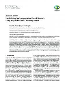
This system was excited by setting u to be a random signal with zero mean uniformly distributed between -2 and 2. Because the current response y(k) depends only on the previous input u(k-1) and output y(k-1) the above problem can be easily visualized in 3D space as shown in figure 2.
3
10 5 0 y(k) -5 -10 5 2 y(k-1)
1
0
0 -1 -5
u(k-1)
-2
Figure 2: The response surface of the nonlinear system (3) to be modeled by the neural network.
3 NETWORK ARCHITECTURE
and sometimes even better than smaller ones. The common goal is, however, to simplify the design without sacrificing its performance. Smaller networks 'assemble' their response surfaces with fewer components coming from each node activation function and therefore their outputs tend to be smoother.
Many neural network applications can be treated as the approximation of a multivariable function. It has been shown theoretically that an architecture with one hidden layer is sufficient to approximate with a desired accuracy any continuous, bounded value function. This kind of approximation makes the somewhat impractical assumption that the number of nodes in the hidden layer can be increased, if necessary, without limits. Therefore, in reality for more demanding applications, neural networks with multiple hidden layers are used.
As the approach presented in this paper allows only shrinkage of the initial topology by removal of redundant links and nodes, in our experiments we have chosen overdetermined networks as a starting point for the optimization procedure. The general architecture under investigation here is the multi-layer perceptron (MLP).
Employing more complicated architectures with several hidden layers inevitably raises questions about the patterns of synaptic connections that should be chosen to fit best a given neural network application. Clearly, the number of units in the network affects its performance; small networks learn slowly or may not learn at all to an acceptable error level. Larger networks usually learn better but such sizes may lead to generalization degradation which is often known as overtraining or overfitting. The correct size of the network is problem dependent and is a function of the complexity of the input-output mapping to be realized by the MLP and the required accuracy. As shown in [13, pp. 180] using cross-validation techniques it is possible to train oversized networks that generalize well
Throughout this work we have not restricted our tests to traditional MLP structures where only neighbouring layers are connected. In general, we assume that pruning can be launched from a layered network with an arbitrary pattern of synaptic links. The only requirement is that an initial network topology must not violate the principle of feedforward architecture, so that no closed or self loops are allowed and all signals inside the network are transmitted in one direction, i.e., from the input to the output layer. An example of a modified MLP is shown in figure 3 (n.b., in general, some connections between nodes may skip the intermediate layers). In all the networks under investigation here, the hidden nodes have the same type of processing nodes
input layer
hidden layers
output layer
∑ ∑ ∑ ∑
∑ ∑
∑ ∑
Figure 3: An example of the kind of feedforward neural network architecture used in the study
4
A)
C)
E)
B)
D)
F)
Figure 4: Different feedforward architectures that may be used to initiate pruning; A only adjacent layers are connected, B - layered architecture with auxiliary, direct links between network input and output, C - layered topology with extra coupling to network output, D - layered topology with extra coupling to network input, E - layered structure with direct links of each hidden layer to network input and output, F - hyper-connected network (all possible connections are allowed).
can, of course, also consider other choices with less links over neighbouring layers, e.g., only output nodes have connections to all other layers. Figure 4 presents various layered network topologies that may be used to initiate pruning.
sigmoid (f(x)=tanh(x)) activation function and the output node has a linear (f(x)=x) transfer function. These are asymmetric functions; as stated in [13, pp. 160] using asymmetric, sigmoid activations for backpropagation networks should ease their training. To increase network capability to approximate non-linear mappings, processing nodes are always biased.
By selecting the topology of an initial network to be pruned we can restrict quite precisely the search space available for an optimization algorithm. For example, if the configuration of the starting network is 2-4-4-1 and connections are allowed only between adjacent layers then a genetic algorithm is able to examine all four layer architectures that have the same or a lesser number of nodes in each hidden layer. Therefore, such topologies as 2-2-2-1 or 2-4-2-1 may be checked because removing certain links in the initial topology leads to deactivation of entire nodes. On the other hand, if for the same configuration of nodes we allow the maximum number of connections (a hyper-connected network) then the search may be also carried through such architectures as 2-3-1 or even 2-1 because it is then possible that whole layers may be abandoned.
Let us assume the initial architecture to be pruned has a full set of links between the nodes of adjacent layers only. After pruning, the resulting network will typically have some unnecessary nodes removed but the number of layers remains unchanged. By choosing topologies where some connections skip neighbouring layers we give the pruning algorithm (at least theoretically) the chance to remove a whole layer. In this paper we therefore also have investigated an initial architecture where all possible connections that do not violate the feedforward nature of the network are allowed (hyper-connected network) so that each layer (starting from the network input side) is connected to all its predecessors. This is an extreme case since it is very likely that we will ask the pruning procedure to remove many meaningless connections. One
1
4 6
3 2
3
4
5
hyper-connected: 2-1-2-1 (connection 4-5 is removed)
5
1
3
1 5 2
6
4
6
hyper-connected: 2-2-1-1 (connection 3-4 is removed)
2
3
hyper-connected network 2-1-1-1-1
1 4
6
2 5
hyper-connected: 2-3-1 (connections 3-4, 4-5 and 3-5 are removed)
Figure 5: Various topologies derived from a hyper-connected network 2-1-1-1-1 by pruning some of its connections.
5
Reset layer numbering for all nodes, Mi = 0; total number of layers Mt = 0.
Choose the first output node.
Mark all nodes of the network as not in use; set layer counter Mc = 1.
Is the choosen node already in use?
Yes
ERROR! Closed loop inside the network.
No
Invoke recursively all incoming nodes with incremented layer counter Mc = Mc + 1.
Mark the current node as the one in use.
Update the node layer number and the total number of layers: if Mi < Mc then Mi = Mc, if Mt < Mc then Mt = Mc.
Yes
Is Mt assigned to nodes other than input ones?
Is any node linked to the current one?
Mt = Mt +1 No Assign all input nodes to the Mt-th layer.
No
Choose the next output node.
Yes
Yes
Is any output node not invoked?
No STOP
Figure 6: A flow chart for the computer routine that arranges nodes of a feedforward network with an arbitrary pattern of connections into layers.
inspection of encoded solutions is a rather laborious task, even for small scale problems (the results presented in this paper involve training 15,000 different networks). Such an algorithm is presented in the form of a flowchart in figure 6. The basic idea behind this method is very simple: assuming that for any node it is possible to obtain a list of units connected to its input at any time, the algorithm recursively invokes all dependent nodes starting successively from the output nodes and assigns incremented layer numbers to nodes as it proceeds deeper into the hierarchically organized feedforward structure. After completing this process the algorithm ensures that the nodes of the input layer (network sensors) are all assigned the highest layer number.
Thus far in discussing various initial topologies for pruning, we have made the simplifying assumption that network hidden nodes are permanently assigned to particular layers. This is always the case for traditional MLPs but for more complicated architectures an association of a given node with a layer is more a matter of mutual dependencies between nodes inside the network. For example, if we remove all links between two hidden layers of a hyper connected architecture 2-4-4-1 then we can arrange this topology into the three layer structure 2-81. Figure 5 presents some rearrangements in network topology that are possible after removing certain synaptic connections from a hyper-connected 2-1-1-1-1 architecture. Although encoding of the hyper-connected architecture with one node in each hidden layer requires the longest chromosome with respect to the number of nodes (for a given framework of network inputs and outputs) this kind of topology has the interesting property of being able to form, as a result of pruning, an arbitrary layered structure with the same or smaller number of originally established hidden nodes.
The algorithm presented in figure 6 arranges network units into layers but the particular locations of nodes inside any one layer remain undefined. In our approach we label each node with an integer number. This number is then used to sort nodes belonging to each layer. Using a modified initial architecture may be also beneficial in other ways. For example, it was observed [26] that if direct connections exist between the network input and output, the process of training was usually substantially shorter and therefore the whole pruning procedure may be completed in less time.
As has been shown, for some architectures, where more connections between layers exist (with some of them skiping adjacent layers), the pruning procedure may cause certain nodes to migrate from one layer to another. Then, the term 'layer' has no precise meaning. We can still use this concept, however, to visualize architectures found by stochastic optimizers. We need an algorithm that is able to arrange nodes into layers automatically, since manual 6
1
1 2
3
3 4
5 2
4
5
1
2
3
4
5
F
0
0
0
0
0I
G G G G G G H
0 L3,1
0 L3,2
0 B3
0 0
0J J 0J
L4,1
L4,2
0
B4
L5,1
L5,2
L5,3
L5,4
0J J
B5 JK
0 0 0 0 0 0 0 0 0 0 L3,1 L3,2 B3 0 0 L4,1 L4,2 0 B4 0 L5,1 L5,2 L5,3 L5,4 B5
L3,1 L3,2 L4,1 L4,2 L5,1 L5,2 L5,3 L5,4 Figure 7: Chromosome construction using strong encoding of the neural network connections.
4 TOPOLOGY ENCODING
are not allowed in feedforward networks. For example, input nodes do not process signals and they cannot have incoming links or biases so the corresponding rows of the connectivity matrix are always zero. Also, within one layer there should be no connections between nodes. This fact, together with the unidirectional transmission of signals from input to output requires at least half the non-diagonal elements of the connectivity matrix to be zero. Violation of these rules leads to obviously invalid topologies. The simplest method to overcome this problem is just to neglect genes whose values cannot be used for some reason. This in fact produces a shortened chromosome with only genes that are significant for the network topology to be pruned. In our experiments we assumed that all processing nodes had biases, so this allows a further exclusion of genes representing these elements. Figure 7 illustrates how the chromosome is built for the case of a simple 3-layer neural network.
For neural network topology optimization performed by genetic algorithms, two main types of encodings (weak and strong) have been used to convert network structures into the form of a chromosome. The weak paradigms require 'interpreters' to translate chromosomes into networks. Such encodings usually store some kind of instruction sets about how to build a neural network rather then direct information about connections. Weak encodings have been reported as being able to produce successful results for constructing large neural networks. Unfortunately, they suffer from several constraints such as search spaces being limited to certain architectures or difficulties in representing detail connections. Such methods usually also require a modification of the standard genetic algorithms operators because different literals in the chromosome string may have different meanings, so for example crossover may not be permitted everywhere in the string. Also the intermediate step of building a network topology from a weak representation makes the relationship between the fitness function and the corresponding chromosome more complicated and it is therefore harder to analyze its impact on the topology search.
The final chromosome representation has several desirable properties. Because all bits are treated uniformly, all genetic operators designed for binary strings can be applied without modification. The chromosome can be used to encode any initial architecture, even with some irregularities. Also, by simply treating the whole chromosome as a series of binary numbers, this encoding can be used with other optimization methods such as simulated annealing. The cost of such flexibility is that, despite the sparse structure of the connectivity matrix, the chromosome length grows rapidly as the network becomes more complicated. For some architectures, this length may approach N 2 2 .
A strong encoding of the network connections establishes a direct relation between synapses and genes in the chromosome string. For this type of representation it is very natural to use a binary alphabet (e.g., 1 - link exists, 0 - no connection). A strong encoding of the connectivity pattern of a multilayer perceptron can then be represented by a N × N matrix (N - number of network nodes including the input layer; in our study the diagonal elements of the matrix refer to the biases of processing nodes and the remaining part encodes synaptic links).
5 SIMPLIFICATION
It is possible to create the chromosome used by the genetic algorithm directly from such a connectivity matrix by concatenating all its elements (more preferably rows since each one encodes full information about incoming links and the bias of a particular node) in one binary vector. However, this representation is overdetermined because some connections that may be encoded using this scheme
Networks created by genetic algorithms or simulated annealing usually contain unconnected nodes or connections that are not used when calculating network responses. A simple example is a 'degenerate' network with no connections to the output layer but fully connected elsewhere so that no signals can be transmitted from the network input to its output. In such a situation the network 7
of figure 9 with biases only on one hidden layer. Here, a simplification procedure would perform the reduction in a somewhat different way. Nodes 3 and 6 are 'degenerate' because they do not receive any input signal (constant zero output is assumed in both cases). Because the output is zero it is not necessary to modify the biases of nodes 7 and 8. On the other hand node 9 has deterministic output sourced from its bias and therefore this node can be reduced to a single bias of the output node 11. Because output node 11 did not have a bias initially it is then automatically added.
architecture could be reduced to two, separate layers, one input layer and one output layer; all existing synaptic connections inside the network are redundant and can be removed. Therefore, in this work a simplification is carried out automatically (before launching the training process) which leaves the input-output mapping unchanged. To explain the method of simplification first we demonstrate how it works for the case of the particular topology shown in figure 8.
3
7
4
8
5
9
6
10
This discussion on feedforward network simplification can be summarized in the form of a flowchart as shown in figure 10. The algorithm is presented in the figure in a rather descriptive manner; its detail implementation heavily depends on how the neural network topologies are stored and maintained by the relevant computer program.
1
11
2
simplification
1
4
5
7
4
8
5
9
6
10
1
7
11
11 2
3
2
8
Figure 8: Application of simplification procedure to a feedforward network with biases on all processing nodes.
simplification
Obviously, in this example node 10 is not functional as it is not used in creating network output and therefore it can be removed together with the connections from node 6. The response of node 3 does not depend on network input because it sources its input signal from bias only and is further modified by a node transfer function and weighted by an outgoing connection before transmitting to node 8. In this situation node 3 behaves as a secondary bias for node 8 and therefore can be combined with it. This results in omitting two redundant parameters (one for the bias and one for the connection weight to node 8) in the network definition. The same procedure might be applied to connections between nodes 6-7 and 6-8 because node 6 has no links from other nodes. A rather different situation is encountered in node 9. Although this node has incoming connections from node 6, its output is also independent from the network input. Therefore, node 9 can be removed from the network without sacrificing its functionality (after correcting the bias of node 11) so finally, the resulting network has only 14 weights (9 connections and 5 biases) instead of 24 weights (15 connections and 9 biases). This reduction in problem dimensionality significantly eases the learning process.
1
4
7
11 2
5
8
Figure 9: Application of simplification procedure to a feedforward network with mixed configuration of biased and unbiased nodes.
6. NETWORK TRAINING Here, neural networks are trained in a batch mode using the RPROP [23, 7] algorithm. This method individually adjusts each weight according to the sign of the weight gradients evaluated during the two most recent iterations. The RPROP algorithm used in our experiments may be summarized as follows: 1.
The first learning iteration is performed using the gradient decent strategy: w j (1) = w j ( 0) + η
In our experiments we have investigated neural networks with all processing nodes biased. In such cases simplification leads to occasionally correcting bias values. However, the method of network simplification can be easily extended to architectures with any configuration of biases. The simplest version can be obtained if we allow the addition of biases to unbiased nodes whenever this kind of action is necessary. To demonstrate the behavior of such an algorithm consider the slightly modified network
∂E ( 0) ∂w j
(4)
Here E is the network error and the learning parameter η is chosen according to the heuristic formula:
8
Calculate output of each node for zero network input.
Yes
No
Is this a marked node?
Yes
Remove all hidden nodes that do not participate in creating network responses.
Does the node receive inputs from marked nodes? No
Does the node have a bias?
Remove from the network all degenerate hidden nodes (those with permanent zero output despite network input and weight configuration).
Create the bias with zero weight.
Yes
Add inputs (scaled by link weights) from all incoming marked nodes to the bias of the currently chosen node.
Mark all hidden nodes where output does not depend on network input.
Choose the first processing network node.
Remove all marked nodes from the network
No
Get the next processing node.
Yes
Is this the last node?
No
Figure 10: A general flowchart of the simplification routine for feedforward neural networks with biased and unbiased nodes.
0.1
η= F
∂E
I
∑ GH ∂w j b0gJK
2
R F ∂E I ∂E | w j (i ) − signG ≠0 J ∆ j (i ), if wj w ∂ ∂ | H j K | ∂E | (7) w j ( i + 1) = S w j (i ), if =0 w ∂ j | |small random value (optional, | , if w j (i ) = 0 |only when training begins) T
(5)
j
2.
During subsequent iterations, step sizes to modify connection and biase values are updated according to the rules:
R ∂E ∂E (i ) ( i − 1) > 0 | min ( ∆ max , ∆ j (i − 1) * u), if ∂ ∂ w wj j | | ∂E ∂E ∆ j (i ) = S max( ∆ min , ∆ j ( i − 1) * d ), if (i ) ( i − 1) < 0 ∂ ∂ w wj j | | ∂E ∂E (6) | ∆ j (i − 1), if ∂w (i ) ∂w (i − 1) = 0 j j T
It is worth noting that the algorithm described by these formulae cannot affect weights which are exactly zero without the optional condition shown in the last equation. When the link weight is zero, the corresponding gradient vanishes and the algorithm has, in general, two choices: do not alter the weight or perform a blind trial in any direction. The occurrence of this situation during the training process is extremely unlikely, except when a given weight is purposely initialized to a null value. This is equivalent to the situation when the link is effectively removed from the network. However, in the experiments presented here we have used the simplification procedure described in the previous subsection to handle trimmed networks.
In these equations the subscript j refers to the specific training data sample and i indicates the current iteration (epoch). In our implementation of the learning algorithm u=1.5, d=0.6, ∆ max =1.0, ∆ min =10 −6 . 3.
The weights are modified by the ∆ j parameter on a
Despite its simplicity, the RPROP algorithm is fast and reliable when compared to other training methods that utilize gradient information. Performing a single iteration is relatively uncomplicated: the main overhead is associated with the evaluation of weight gradients in the backpropagation scheme. Because topology optimization using a genetic algorithm involves the training of several hundred different topologies we have modified the computation of weight gradients to make training even more efficient.
regular basis only if the corresponding element of the gradient vector is non zero, i.e.:
9
10
0
MSE error
10
(C)
-1
(B) (A)
10
-2
10
-3
0
500
1000
1500
2000
4000
4500
5000 epoch
Figure 11: Changes of the learning (A) and validation (B) errors during training. The curve C is the sum of traces A and B.
network performance periodically during training to assure that further training improves generalization as well as reduces learning error (the so called cross-validation technique). For this purpose an additional set of validation data, independent from the main training pool is used. In a typical training phase, it is normal for the validation error to decrease. This trend may not be permanent however: at some point the validation error usually reverses or its improvement is extremely slow. The training process should then be stopped. Figure 11 presents example traces of learning and validation errors as they vary during training.
As the network error approaches zero, for some training samples the corresponding gradient is vanishingly small. This happens more frequently as the training progresses and the network becomes able to learn the desired patterns. At some point backpropagating very small errors may be counter-productive because the associated updates of the batch gradient ∇E are then negligible. In the training process used here, we have set a threshold for the data samples which are used to calculate the gradients; if the relative output error for a given training point is less than a threshold β , (typically β = 0. 5 ) the partial update of the batch gradient is assumed to be zero, i.e.: NL
Rx , if Ei ≥ β Etrg ∂Ei I J , ϕ(x) = S H ∂w K T0 , if Ei < β E trg F
∇E = ∑ ϕ G i =1
Detecting the point of minimal training and validation error is not an easy task. Figure 11 shows that during the learning process we cannot expect smooth curves that easily allow us to locate the point of a minimal validation error (curve B) or the sum of learning and validation errors (curve C). This is exacerbated by the shifting nature of the validation error. Also, when the RPROP algorithm is used, the learning error may occasionally increase, because this algorithm does not check if every iteration causes the learning error to reduce before accepting a new weight adjustment. Some training algorithms are more restrictive and discard weight updates that cause the learning error to rise. Others may purposely allow an increase in learning error to some extent because this helps the learning procedure to escape from shallow, local minima of the error surface. This, however, make the changes of the validation error even more irregular and difficult to utilize.
(8)
In this formula E trg is the acceptable training error level. The approach described typically accelerates evaluation of the network gradients. As the training converges, the execution of subsequent iterations takes less time because the samples for which the error is already small enough are rejected. We have found that this method also helps to achieve a better generalization since the training algorithm has the capability to focus training on samples with the higher errors and to neglect areas where the network response surface matches the desired output pattern well. Although this modified gradient evaluation has been used in conjunction with the RPROP algorithm, the same modification may be applied to virtually any training paradigm that utilizes gradients. Our brief experiments indicate that such training methods as Super-SAAB, DeltaBar-Delta, Silvia-Almeida or adaptive learning with momentum [23, 7] are stable and work well with this modification.
Typically, at the beginning of training, the validation error oscillates rapidly. Later, the training process stabilizes and the changes in validation error become smaller. Instead of a clear increasing trend in the validation error, that characterizes overfitting, it may then start to wander around some constant value. In such a situation the magnitude of the generalization error may not be the best indication of when to stop training. Consequently, we have used the number of subsequent, unsuccessful training epochs as a stopping criterion. An unsuccessful training iteration occurs when:
Another important issue associated with network training is the termination criterion. The main goal of training is to minimize the learning error while ensuring good network generalization. It has been observed that forceful training may not produce networks with adequate generalization ability although the learning error achieved is small. The most common remedy for this problem is to check the
F G H
10
E L EV + N L NV
I J K i
F
≥G H
E L EV + N L NV
I J K i −1
(9)
samples is sufficient. Such values are used for fine training of a single network. Because training using big data sets is time consuming, in the present work we have used the substantially reduced number of 25 input/output pairs for training to estimate the usefulness of a particular neural network. Then, after completing a topology optimization, we trained the best performing network on a larger number of data samples.
In our implementation of the training algorithm, network training is stopped when 250 consecutive iterations are unsuccessful. As with other rank based methods, this stopping condition is robust and easy to implement. Of course, setting the number of unsuccessful iterations to 250 epochs (or more) does not guarantee that there would not be any successful steps ahead if training continued. When the learning process is saturating, new, successful iterations are typically encountered less and less frequently. Of course, at some stage a training algorithm may recover from some local attractor and accomplish further error minimization, but we require it should occur within a certain number of trials. Therefore, the number of unsuccessful training iterations defines a cost limit on achieving error minimization. Obviously, when training is stopped according to this criterion, the final set of network weights does not correspond to the best result found. It is therefore necessary to store the weight values in a separate array every time a successful training step is made. At the end of the training process the best set of network weights is then recalled.
As the number of training samples is one of the major key issues that determines the time and CPU resources required to complete the topology search, for some applications where more, possibly noise free data are available, the training set could be reduced by estimation of the novelty of each training pattern. Such a technique is for example discussed in [5]. In our two experiments, initial unpruned neural networks with 177 weights (152 link weights, 25 biases) and 183 weights (164 link weights, 19 biases) are used, respectively. All the networks were allowed to train for a maximum of 5,000 epochs. Learning was stopped earlier if the network achieved an output error of less than 0.001 per data sample used during training. For moderately pruned networks and 25 training samples, convergence was usually achieved in many fewer cycles. After completing the training phase, networks were validated using 100 previously unseen data points.
In some cases the training process may be obstructed by the total inadequacy of a network architecture to learn the desired patterns or by saturation of network nodes. If all elements of the weight gradient are very small then the training algorithm cannot obtain reliable indications of where the search should be directed. This situation is rare but if it occurs, training may be executed over a very large number of epochs without any real chance of obtaining a useful result. To provide early detection of this problem, the training algorithm evaluates the L2 norm of the batch gradient every 100 epochs. If the norm is smaller than 10 −6 , the training process is aborted.
7 FITNESS FUNCTION In our study optimal network design corresponds to the global minimum of a fitness function. When constructing this function we have tried to avoid incorporating explicitly parameters that are not directly associated with neural network topology, such as the number of cycles required to train the network or the speed of convergence (these values can loosely characterize a training algorithm as well). The main factor used for the fitness function is the networks ability to generalize unseen patterns. For this purpose we have used a relatively large number of input-output patterns as a validation test in comparison to the training subset. To create a strong selective pressure that favours smaller networks, a so called effective number of active connections or number of connections in the simplified network is also included in the fitness function as a parameter describing the network size. Throughout these experiments we utilized two types of fitness function:
Finally, it is worth emphasizing that the RPROP algorithm is a local optimization method. In practice, this means that the final results of training may vary as the initial weight settings are changed. Typically, the error surfaces of feedforward networks have many local minima. This means that the training process is sensitive to its starting point. Despite recent progress in finding the most appropriate weight initialization that would help a training method to find near optimal solutions, the most widely adopted approach still utilizes random weight initialization. Our experiments with stochastic optimizers employed to design neural networks show that using different random starting points for training a given network at each stage of the topology search severely deceives such methods [24]. Under these circumstances even the best architecture found so far by a topology optimizer may perform quite indifferently when trained in the next generation from another starting point. For this reason a fixed initial value was assigned to each bias and weight to reduce fluctuation in evaluation of similar neural networks.
F
F ( ⋅) = λ G H
E L EV + N L NV
I J K
+
LA Lmax
(10)
LA I J Lmax K
(11)
and F
F ( ⋅) = G H
A rule of thumb for choosing the size of training set to achieve good neural network generalization is to select the number of training patterns to be between 10* N w and 20* N w (where N w is the total quantity of weights in the network) although sometimes a smaller number of data
E L EV + N L NV
IF J G1+ KH
where E L and EV corresponds to sum square error for learning and verification, respectively and N represents the number of data patterns used in each stage. L A is the number of connections after network simplification and Lmax is the maximum number of allowed links (the length 11
10 10 10 10
2 1
0
10
1
0
-1
-1
10 50
100
150
0
200
2
50
100
150
200
1
10
(B) 10
(C)
10
0 10
2
10
(A)
(D)
1 0
10 10 10
0
-1
-1
0
10 50
100
150
200
0
50
100
150
200
Figure 12: A comparison of fitness values evaluated for 200 neural networks by different training algorithms: A - gradient decent with adaptive learning rate and momentum, B Levenberg-Marquardt, C - RPROP, D - RPROP averaged over five independent runs.
of the chromosome used to encode the initial topology). The purpose of the constant λ in equation (10) is to scale the sum square errors to the same order (10 −1) as the component indicating network complexity ( L A Lmax ).
Evaluating a given network simply on learning results and validation tests has several other drawbacks. For example, using a small number of samples in both phases speeds up the optimization process but may result in removing synaptic connections too forcefully since the limited number of measurements might not provide enough evidence to justify the importance of some links. On the other hand, using a larger quantity of data to evaluate the network may mean that bigger networks could be trained more precisely than smaller ones and therefore the pruning process would be reluctant to remove links. This may especially be the case when employing cross-validation techniques. Such methods use more sophisticated strategies during training: as some, particularly oversized, networks exhibit a tendency for overtraining which is manifested in an almost perfect fit to the training data but much larger validation error, it is possible to perform a periodic check of the overall network performance during the training phase and terminate it (even before reaching the desired learning error) if validation results are continuously deteriorating. As a result we may expect to obtain smaller values of the b E L N L + EV NV g component of the objective functions and consequently abate the selective pressure against bigger architectures. This could be balanced by a modification to the penalty factor representing network relative size as follows:
For networks that were trained successfully E L (the network's ability to memorize training data) is negligible. In such cases it is the performance during verification (its generalization ability) and the size of the network that control the value of the fitness. Only if the network could not be trained is EV NV expected to be high; E L N L then further worsens the fitness to ensure that a given solution would be likely to be rejected by the optimization procedure. In equation (11) the second element b1+ L A Lmax g may be interpreted as a penalty coefficient; as the network gets smaller this factor approaches 1 while for a fully connected network it is 2. This version of fitness function avoids the use of the parameter λ which has to be adjusted before launching topology optimization but it limits the magnitude of the complexity penalty. Although these formulae for the fitness functions are relatively simple their values depends on several 'hidden' factors that are not directly associated with network topology. For example, the choice of learning algorithm or even its internal parameters influence the value of fitness. Under one set of circumstances the network may be trained successfully while in another the algorithm may fail to converge and therefore the network would be considered useless. Figure 12 shows the value of fitness function (11) evaluated for the same set of 200 networks using different training algorithms (to generate these networks the chromosome was treated as a binary number that was simply incremented). Clearly, the same networks would appear differently to a topology optimizer when different training algorithms were employed. (It should be noted that the curves displayed on this figure do not represent the true function to be optimized which is a problem spanned over mulit-dimensional binary space. This is only a oneto-one comparison of the fitness function values calculated for the same neural networks and the same initial weight conditions.)
F
F ( ⋅) = G H
E L EV + N L NV
I J K
R
F G1 + H
LA Lmax
I J K
S
(12)
where S is a constant parameter (S > 1. 0 , stronger tendency to remove synaptic links, 0. 0 < S < 1. 0 - weaker selective pressure). The second parameter R ( R ≤ 1) may be also used to scale the network performance evaluation. In some cases setting these parameters to other values than assumed here as default ( R = 1, S = 1) may considerably improve the efficentcy of the topology search [24]. In some cases, especially when the initial, unpruned network is small, this penalty factor may be difficult to adjust precisely using the parameter S. The penalty function may still overly reward small networks and
12
R1, if Fi ≤ Fi −1 | Pi (⋅) = S F 1 Fi − Fi −1 I exp − , if Fi > Fi −1 | GH T F1 − F0 JK T
remove too many links. In such cases, a modified complexity penalty factor Θ can be applied: F
RL
H
EV E I + LJ NV N L K
F G H
EV E I + L J Θ b L A Lmax g NV N L K
F (⋅ ) = G
M1 + b γ M N
F
− 1g G H
LA I J Lmax K
SO
P P Q
=
(14)
The probability of accepting an unsuccessful mutation depends on the relative change of the objective function Fi (⋅) and a parameter T (the annealing temperature) that varies throughout the search. At the beginning of the search T is relatively high so that most of the steps are accepted. At this stage the method is similar to a random search. As the search progresses the annealing temperature is reduced several times to approach a small, positive value or zero just before termination. Then the process resembles the random descent strategy. For 500 allowed evaluations of the objective function the number of annealing temperatures, N T , was chosen to be eight and the temperature was decreased at intervals chosen according to the formula:
(13)
R
The parameter γ ( γ ≥ 1) affects the maximum value of the complexity penalty while the exponent S controls the shape of the function Θ: for S approaching unity the penalty is close to linear but as S increases a stronger penalty is applied to the biggest networks leaving smaller and medium size architectures relatively unpenalized. This more sophisticated objective function is not pursued further here.
8 STOCHASTIC OPTIMIZERS
bNT
Tj = τ w
The genetic algorithm tested here uses four basic operations as described in [11], i.e., multi-point crossover (crossover probability, PC = 0. 8), mutation ( PM = 0. 005), inversion ( PI = 0.8 ) and selection. The selection† scheme is generational, linear ranking and extinctive, allowing the best 80% of the current population to breed and discarding the remaining 20% of chromosomes. It is also 1-elitist so the top performing individual of each generation is assured of being included in the next population. To prevent the genetic algorithm from being dominated by a few moderately good designs that may block further exploration of the search space a fitness sharing scheme is employed as described in [16, 11]. This method performs a cluster analysis of the current population and modifies the raw objective function so that the chances of creating individuals in overcrowded regions are reduced. A somewhat opposite operation, inbreeding, is launched if, despite the niche penalty, a particular cluster remains numerous.
τc − jg
,
j = 1,..., N T
(15)
where τ w and τ c are the control parameters of the cooling schedule; τ w regulates the range of annealing temperatures while τ c shifts this range to encompass lower or higher values. Here τ w was set to 5 and τ c to 2.
9 EXPERIMENTAL RESULTS Figure 13 illustrates the distribution of fitness for 2,500 networks derived by randomly pruning the fully connected architecture 2-8-8-8-1 (fitness function (10)). A similar type of distribution was encountered when random pruning was started from the hyper-connected network 2-6-6-6-1 (fitness function (11)). It is important to note that, as we search for a superior network (smaller fitness function), the expected number of improved solutions grows at first (!) to reach a maximum; then the number of excellent topologies is sharply decreasing. This demonstrates the well known robustness of neural networks which are able to function even when partially damaged.
Here a population size of 50 chromosomes was used by the genetic algorithm. The method was initialized with 49 randomly created individuals in addition to the one chromosome having all genes set to one that corresponds to an unpruned network. The number of generations was set to ten.
Perhaps surprisingly, the bar graph of figure 13 suggests that for a random search it is quite difficult to find a network with the worst fitness function (or close to the worst) since the number of networks with such deteriorated performance decreases in an exponential fashion. On the other hand, many such architectures can be readily constructed by hand.
For the simulated annealing method the same strong encoding was used and the unpruned network architecture was selected as a starting point. The routine [16] uses fixed rate random mutation with probability 0.1 to drive the search. If modification of the current solution is successful then the new point is always accepted. When the i-th iteration fails to lower the objective function then the proposed step may be rejected or not. A decision to switch to the new point is made with a probability Pi (⋅) defined as follows:
The distribution presented in figure 13 shows that the probability of finding a solution better than the fully connected, unpruned network is relatively high. As a result, even a few random samples can be beneficial. This situation may be misleading when reviewing the results of optimization without comparison to other methods. One may expect that some optimization strategy that is more sophisticated than a random search works, but only comparison with the latter reveals if this initial hypothesis is correct.
† Terminology used to describe selection follows definitions presented by Bäck and Hoffmeister in [1].
13
250 number of networks 200
150
100 unpruned network average fitness 3.46 50
0
0
2
4
6
8
fitness function (eq. 4)
Figure 13: The performance distribution of 2,500 neural networks obtained by randomly pruning a fully connected MLP 2-8-8-8-1.
traces show more successful steps in searching for better network structures than a single run which typically ended with only 2 to 5 improvements after the first rapid fall.)
The difference in value of the fitness function between the most superior networks found and those with slightly worse performance, but which form the most numerous group, is clearly small. This further justifies the importance of precise evaluation of network fitness as even a small amount of noise introduced during training of the best networks may result in totally erroneous classifications. Inaccurate training may then potentially mislead the search being conducted by genetic algorithm or simulated annealing and produce less reliable results. In the presence of such noise, it may be expected that increasing the population size of the genetic algorithm should help to prevent it from being deceived. For simple measurements, contaminated by uncorrelated, zero mean noise, increasing the number of trials and averaging the results reduces the disturbance. However, here it is arguable that a similar effect takes place when more, less accurate network evaluations are used since the character of the noise introduced during the network training phase is unknown.
The figures suggest that, for our problem, genetic algorithm or simulated annealing optimization are, on average, able to find comparable solutions using half or less the iterations required by a random search. A factor of only two increase in convergence speed over an unguided search may seem disappointing at first, but this result should be interpreted carefully. The most significant fact is that both genetic algorithm and simulated annealing were able to find solutions that could not be discovered by a random search at all. If we take into account the fact that the expected number of excellent networks decreases very rapidly and that the search was conducted in a noisy environment the final optimization results seem quite encouraging. Figures 16 and 17 visualize the generalization ability of the unpruned fully connected network 2-8-8-8-1 and the best network found by the genetic algorithm (appendix A.1, topology #4). The pruned network, besides its overall smaller error, offers a better generalization than its unpruned counterpart after training, even with only 25 samples. The generalization of the pruned network continues to improve using bigger training data sets while for the fully connected network the error surface then
Figures 14 and 15 compare the progress made during topology pruning of fully and hyper-connected neural architectures, respectively. All the traces exhibit initial, rapid changes in the fitness. However, after 50-100 iterations the search becomes more arduous as the number of better networks sharply decreases. (N.b., these results were averaged over five independent runs for each optimization method. Consequently, the corresponding
fitness function
0.8
0.8 fitness function
0.75 0.7 RN 0.7
RN GA
0.6 SA
0.65
SA GA 0.5
0.6
0.55 0.4 0.5
0
100
200
300
400
0
500
100
200
300
400
500
number of iteretions
number of iterations
Figure 14: Topology pruning of the fully connected neural network (2-8-8-8-1) using genetic algorithms (GA), simulated annealing (SA) and random search (RN). Fitness function defined by equation (4).
Figure 15: Topology pruning of the hyper-connected neural network (2-6-6-6-1) using genetic algorithms (GA), simulated annealing (SA) and random search (RN). Fitness function defined by equation (5).
14
method
topology: 2-8-8-8-1 fully connected
training
topology: 2-6-6-6-1 hyper-connected
data
initial
pruned
initial
pruned
25
1.1307
0.2188(1)
2.1491
0.1648(3)
100
1.0076
0.1202
0.6958
0.1074
25
1.7663
0.2311(2)
1.9267
0.2341(4)
100 0.2813 0.2452 (1) - appendix A.1, network #4, (2) - appendix A.2, network #3, (3) - appendix A.3, network #4, (4) - appendix A.4, network #2.
0.8004
0.0804
GA SA
Table 1: Performance comparison of the best networks found in each topology optimization test (the numbers in the table are averaged validation taken across 625 equally spaced points (25x25 grid) of the network input domain after training from the initial weights used in the optimization searches).
shows the typical attributes of overtraining (i.e., a bumpy landscape).
architecture may help find better performing networks than those produced from a standard MLP.
Table 1 summarizes the best results obtained by the topology optimizers. It lists square sum errors averaged over 625 equally spaced points (25 × 25 grid) of the rectangular area, −2 ≤ u ( k − 1) ≤ 2 , −5 ≤ y ( k − 1) ≤ 5 , where neural network modeling (eq. 3) is applied. As these points are different from the training and validation data so the corresponding errors can be used to make an independent comparison of the various networks trained with 25 and 100 data samples. The results suggest that initializing the pruning process from a hyper-connected
When the pruned network is trained with more data it may be expected that its overall performance would improve. However, the best network obtained from a fully connected architecture by simulated annealing (appendix A.2, topology #3) behaves in somewhat different way. Although its structure is similar to the network found using the genetic algorithm (appendix A.1, topology #4), the performance does not get better when larger numbers of training data are used. Consequently, the corresponding response surface (figure 18-B) gradually loses relevant
(A)
e(k)
(B)
10
10
5
5
0
0
e(k)
-5
-5
-10 5
-10 5 2
2
1
0
0
y(k-1)
u(k-1)
-1 -5
1
0
0
y(k-1)
-1
-2
-5
u(k-1)
-2
Figure 16: Difference between the neural network and nonlinear system outputs; A - fully connected neural network 2-8-8-8-1, B - the best network structure obtained after pruning by genetic algorithm - network #4, appendix A.1. Both networks were trained using 25 input-output pairs. (A)
e(k)
(B)
10
10
5
5
0
e(k)
-5
0 -5
-10 5
-10 5 2 y(k-1)
2
1
0
0 -1 -5
y(k-1)
u(k-1)
1
0
0 -1 -5
-2
-2
Figure 17: Evidence of the better results for generalization ability of the networks found as the result of pruning. The charts show results for the same networks as in figure 16 but their training was performed using 100 data points instead of 25.
15
u(k-1)
(A)
(B)
10
10
5
5
0
0
y(k)
y(k) -5
-5
-10 5
-10 5 2 y(k-1)
1
0
0 -5
-1
y(k-1) u(k-1)
-2
1
0
0 -5
-1
2
u(k-1)
-2
(C)
(D)
10
10
5
5
0
0 y(k)
y(k) -5
-5
-10 5
-10 5 y(k-1)
1
0
2 y(k-1)
0 -5
-1 -2
u(k-1)
1
0
2
0 -5
-1 -2
u(k-1)
Figure 18: Response surfaces of the best networks obtained in each topology optimization test after training with 100 data points; A - network #4, appendix A.1 (GA, fully connected start), B - network #3, appendix A.2 (SA, fully connected start), C - network #4, appendix A.3 (GA, hyper-connected start), D - network #2, appendix A.4 (SA, hyperconnected start).
search was stuck in a saddle point or shallow local minimum.
detail folds and the network 'generalization' becomes inaccurate. We have found that further increasing the number of training data, e.g., to 500 or 1000 samples, may cause a similar effect for the other pruned architectures. This suggests that the number of data points used for network testing may affect the final pruning results. Also, it seems that the hypothesis: 'if a given network performs well for a small number of training points, it will operate even better after training with more data' may not be extended too far.
To assure that the topology optimization search was guided toward smaller networks we have explicitly introduced penalty factors that worsen fitness as networks become more complex. In this way, the criteria of optimality defined here implies that the best networks should be a compromise between size and performance. Other pruning techniques, e.g. OBD or OBS, deal with a similar type of dilemma: they attempt to estimate the consequences of removing every connection inside a fully trained network and accept only those changes that are least disruptive, but not necessarily beneficial. In our approach, the balance between complexity and performance can be regulated at the level of the fitness definition but care must be exercised when setting values since the network performance depends also on other 'hidden' aspects of the optimization problem, such as the number of training and validation points, the initial unpruned topology, the particular training algorithm and the overall training strategy.
10. CONCLUSIONS We have demonstrated that it is possible, using stochastic optimization methods, to find neural networks with good generalization features even using comparatively small numbers of data points for training and verification. The time consuming nature of the evaluation of each design considered led us to use such trimmed data pools. These are, nonetheless, shown to be sufficient for the experiments carried out. Moreover, for some neural network applications, the limited number of available measurements may well restrict training in this way.
A general simplification procedure for feedforward networks (as generated by the stochastic topology optimizers) has been proposed for three main reasons: (i) to speed up the training phases, (ii) to eliminate useless connections or those with duplicated functions and (iii) to asses the actual architecture complexity.
Since the problem under investigation, i.e., nonlinear identification, is closely related to the interpolation task the main measure of a network's usefulness is its ability to generalize. The total sum squared training error is less meaningful; a lack of convergence within a maximum number of epochs may arise because of the deficiencies of a particular architecture but it could also show that the initial starting point for training was placed too far from the optimum or the choice of training algorithm was not suitable for a given shape of error surface or the training
Although the number of tests performed here does not allow any conclusive, general statement to be made, a closer examination of the test problem reveals that, in this case, neural network topology pruning is basically a two stage process. During the first period, rapid improvement is observed which is associated with the underlying 16
[13]
problem (architecture robustness rooted in network redundancy) and which should not be used to judge the efficiency of a particular optimization method. The second, less spectacular, stage of slow and arduous convergence is the phase when the optimizers are achieving real gains.
[14]
[15] ACKNOWLEDGMENTS We would like to thank Prof. Andrzej Cichocki from the Warsaw University of Technology (Poland) and Laboratory of Artificial Brain Systems FRP RIKEN (Japan) for his encouragement and suggestions.
[16]
[17] REFERENCES [1]
[2]
[3]
[4]
[5]
[6]
[7]
[8]
[9]
[10]
[11]
[12]
Bäck T., Hoffmeister F., Extended Selection Mechanisms in Genetic Algorithms, Proc. 4th Int. Conf. on Genetic Algorithms, Morgan Kaufmann, 1991, pp. 92-99. Beaufays F., Abdel-Mogid Y., Widrow B., Appication of Neural Networks to Load-Frequency Control in Power Systems, Neural Networks, Vol. 7., No. 1., 1994, pp. 183-194. Bhat V.H., Minderman A.P., McAvoy T., Wang N. S., Modeling Chemical Process Systems via Neural Computation, IEEE Control Systems Magazine, April 1990, pp. 24-29 Billings S.A., Jamaluddin H.B., Chen S., Properties of neural networks with applications to modeling non-linear dynamical systems, Int. J. Control, 1992, Vol. 55, No. 1, pp. 193-224. Bishop C.M., Novelty Detection and Neural Network Validation, IEE Proc.: Vision, Image and Signal Processing, 141 (4), pp. 217-222. Chen S., Billings A., Neural Networks for nonlinear dynamic system modeling and identification, Int. J. Control, Vol. 56, No. 2, 1992, pp. 319-346. Cichocki A., Unbehauen R., Neural Networks for Optimization and Signal Processing, 4th ed., Wiley & Sons, 1994. Eigel-Danielson V., Augustejin M. F., Neural Network Pruning and its Effect on Generalization some experimental results, Neural Parallel & Scientific Computation 1, 1993, pp. 59-70. Evans, J.T., Gomm J.B., Williams D. ,Lisboa P.J.B., To Q.S., A practical application of neural modelling and predictive control, chapter 6 in Application of Neural Networks to Modelling and Control, Page G.F, Gomm J.B., Williams D. (eds.), Chapman & Hall, 1994 Fahlman S. E., Lebiere C., The cascade-correlation learning architecture, Technical Report CMU-CS90-100, Carnegie Mellon University, 1990. Goldberg, D. E., Genetic Algorithms in Search, Optimization and Machine Learning, AddisonWesley, 1989. Hassibi B., Stork D. G., Wolff G. J., Optimal Brain Surgeon and General Network Pruning, 1993 IEEE International Conference on Neural Networks, Vol. 1, pp. 293-299.
[18]
[19]
[20]
[21]
[22] [23]
[24]
[25]
[26]
[27]
[28]
17
Haykin S., Neural Networks - A Comprehensive Foundation, Macmillan College Publishing, 1994. Hunt K.J., Sbarbaro D., ¯bikowski R., Gawthrop P.J., Neural Networks for Control Systems - A Survey, Automatica, Vol. 28, No. 6, 1992, pp. 10831112. Jutten C., Learning in Evolutive Neural Architectures: An Ill - Posed Problem?, From Natural to Artificial Neural Computations, Int. Workshop on ANN, Springer-Verlag, 1995, pp. 361-371. Keane A..J., The Options Design Exploration System, Reference Manual and User Guide, 1994, available by Internet, http://www.eng.ox.ac.uk /people /Andy. Keane /options.ps. Keane A.J.., Experiences with Optimizers in Structural Design, Proc. Conf. on Adaptive Computing in Engineering Design and Control, Plymouth 1994, pp. 14-27. Kuscu I., Thornton C., Design of Artificial Neural Networks Using Genetic Algorithms: review and prospect, Cognitive and Computing Sciences, University of Sussex, 1994. Miller G.F., Todd P.M., Hegde S.U., Designing neural networks using genetic algorithms, Proc. 3rd Int. Conf. on Genetic Algorithms, Morgan Kaufmann, 1989, pp. 379-384. Naidu R.S., Zafiriou E., McAvoy T.J., Use of Neural Networks for Sensor Failure Detection in a Control System, IEEE Control Systems Magazine, April 1990, pp. 49-55. Narendra K. S., Parthasarathy K., Identyfication and Control of Dynamical Systems Using Neural Networks, IEEE Trans. on Neural Networks, Vol. 1, No. 1, 1990, pp. 4-27. Reed R., Pruning Algorithms - A Survey, IEEE Trans. on Neural Networks, vol. 4, No. 5, 1993. Schiffmann W., Joost M., Werner R., Optimization of the Backpropagation Algorithm for Training Multilayer Perceptrons, Technical Report, University of Koblenz, 1992. Stêpniewski S.W., Keane A.J., Topology design of feedforward neural networks by genetic algorithms, (submitted). Wang D., Chai T., Multivariable Adaptive Control of Unknown Nonlinear Dynamic Systems Using Neural Networks, Proc. 33rd Conf. on Decision and Control, Lake Buena Vista, FL, 1994, pp. 25002505. Whitley D., Starkweather T., Bogart C., Genetic Algorithms and Neural Networks: optimizing connections and connectivity, Parallel Computing 14, 1990, pp. 347-361. Willis M.J., Massimo C., Montague G.A, Tham M.T., Morris A.J., Artificial neural networks in process engineering, IEE Proc. Pt. D, Vol. 138, No. 3, 1991, pp. 256-266. Yaw-Terng Su, Yuh-Tay Sheen, Neural Network for System Identification, Int. J. Systems Sci, Vol. 23, No. 12, 1992, pp. 2171-2186.
APPENDIX A.1 FULLY CONNECTED START
GENETIC ALGORITHM INITIAL ARCHITECTURE AND BEST RESULTS IN EACH OF FIVE RUNS unpruned network 3
11
(1)
19 4
4
12
20
5
13
21
6
14
22
11
1 1
19 6
13
27 27
7
15
23
7
15
2 2
8
16
24
9
17
25
10
18
26
23
10
average fitness = 3.4616
17
fitness = 0.5506 (iteration 420) (2)
(3) 5
4 14
12 6
1
1 6 7 15
23
27
15
23
27
8
7 2
2 9
17
17
10 10
fitness = 0.5160 (iteration 46)
fitness = 0.5165 (iteration 279) (4)
(5) 3 11
5 4
13 1
1
6
12
24
5
7
14
23
7
27
14
27
8 2
2
9
15
26
9
15
16
10 10
fitness = 0.4852 (iteration 475)
fitness = 0.5528 (iteration 455)
18
APPENDIX A.2 FULLY CONNECTED START
SIMULATED ANNEALING INITIAL ARCHITECTURE AND BEST RESULTS IN EACH OF FIVE RUNS unpruned network 3
1
11
19
4
12
20
5
13
21
6
14
22
1
27
2
(1)
7
15
23
8
16
24
9
17
25
10
18
26
2
average fitness = 4.1458
3
11
4
12
5
13
8
16
9
17
25
27
fitness = 0.5361 (iteration 208) (2)
(3)
11 3 3
1
12 12
13
1
22
5 15
6 14 7
27
21
27
15 16
8 2
16
9
2
23
9
17
17 10
18
fitness = 0.5836 (iteration 321)
fitness = 0.4542 (iteration 453) (4)
(5) 3
3
11 12 4 1
1
21
5 15
7 17
19
8
27
8
16
2
2
23
9
9 18
18 10
10
fitness = 0.4995 (iteration 212)
fitness = 0.4937 (iteration 458)
19
27
APPENDIX A.3 HYPER-CONNECTED START
GENETIC ALGORITHM INITIAL ARCHITECTURE AND BEST RESULTS IN EACH OF FIVE RUNS unpruned network 3
9
15
4
10
16
(1) 10
1
3
9
1
13 5
11
17
21 21 15
6
12
18 2
6
11
2 7
13
19 18
8
14
20
average fitness = 3.7690
fitness = 0.3637 (iteration 380) (2)
3
(3)
4 5 3
1 1 6
11
10
9
21 4
7
21
14
2 2
14
11 8
6
19
fitness = 0.3453 (iteration 320)
fitness = 0.3766 (iteration 344) (4)
3
(5)
11
11
1
1
5
12
19
21
14
12
2
2 7
3
5
21
16
14
13
fitness = 0.3325 (iteration 463)
fitness = 0.3346 (iteration 164)
20
APPENDIX A.4 HYPER-CONNECTED START
SIMULATED ANNEALING INITIAL ARCHITECTURE AND BEST RESULTS IN EACH OF FIVE RUNS unpruned network 3
9
(1)
15
9 3
4
10
16
10
1
1
15 4
5
11
17
6
12
18
11 21
21 12 6
2
2 7
13
19
8
14
20
18 13 7 14
average fitness = 4.3133
fitness = 0.3981 (iteration 172) (2)
(3)
9
10 15
1
4
10
12
2
8
5
3
1
17
21
12
6
13
9
2 20
13
21
14 7
11
14
19
fitness = 0.3616 (iteration 492)
fitness = 0.3951 (iteration 392) (4)
3
(5)
9 4 15 1
1
4
10
5
11
6
12
9
12
5 19
2 2
21
21
11
19
8 20 8
13
fitness = 0.4309 (iteration 470)
fitness = 0.3722 (iteration 114)
21