Image Registration: Color Image Synthesis from Data Obtained from ...

Image Registration: Color Image Synthesis from Data Obtained from Satellites Pushbroom Cameras Dmitry V. Yurin Laboratory of Mathematical Methods of Image Processing, Department of Computational Mathematics and Cybernetics, Moscow State University, Moscow, Russia [email protected]

Abstract The problem of image registration is discussed. Firstly, the well known Reddy-Chatterji algorithm is revised. It is shown that the speed may be dramatically increased by using Hartley transform instead of Fourier transform, especially when registration is required for more than two images. Secondary, a new registration algorithm is proposed for images obtained from pushbroom cameras that is based on Hartley transform and fast Hough (Radon) transform. The issue of aliasing and artifacts suppression is treated. Two cases have been considered: approximately linear correlated spectral bands and without this assumption. Registration obtained is refined with optical flow technique up to subpixel accuracy Keywords: Image registration, pushbroom camera, Fourier transform, Hartley transform, Hough transform, Radon transform, affine model.

One row of image is obtained by reading data from a sensor line at a time. Different image rows are obtained by reading data from the line sensor in time intervals, the satellite moves and hence different Earth surface lines become visible. Some geometric properties of pushbroom cameras are investigated in [8-11]. To obtain very wide images such sensors can be assembled as stairs of line sensors. One of the problems of synthesis color (or pseudo color) images is that due to line sensors related to different spectral bands are spased in the focal plane, each time they see different lines of the Earth surface. In section 2 we remind definitions and properties of Fourier and Hartley transform. In section 3 we review Reddy-Chatterji algorithm [1]. In section 4 we modify it using Hartley transform, discuss some implementation issues, and extend it for no linear correlated spectral bands and color images. In section 5 we propose a new registration algorithm for pushbroom cameras. Section 6 presents some results.

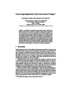
1. INTRODUCTION Image registration is an area of intensive research in computer vision [1-7]. One possible application of image registration is creation of mosaics from satellite images [1-6]. Pushbroom cameras are widely used for high resolution satellite imaging. Such cameras are composed from one or more CCD line sensors placed at focal place of the camera (see Figure 1).

Focal plane

2. FOURIER AND HARTLEY TRANSFORMS Fourier transform

r F (ξ )

r F (ξ ) = ∫

r f (x) is defined as [12]: r r r r f (x)exp(2πix T ξ )dx (1) of function

Inverse Fourier transform is:

r r r r r f (x) = ∫ F (ξ )exp(-2πix T ξ )dξ

(2)

Amplitude or module of Fourier transform is:

r r r r M ( ξ ) ≡ F (ξ ) ≡ F (ξ ) F * (ξ ) Push broom camera

(3)

Where symbol * denotes complex conjugation. Fourier transform of real-valued function is a complex-valued function with properties:

CCD line sensor

r r r r F ( ξ ) = F * ( − ξ ) , M (ξ ) ≡ M ( − ξ )

(4)

If we compose a complex-valued function from two real-valued

r

r

r

functions f ( x) = f 1 ( x) + if 2 ( x) , their Fourier transforms can be extracted from Fourier transform of this complex valued function using property (4) as

Building Earth surface Figure. 1. Multiband pushbroom camera and shooting geometry

[ [

] ]

r r r 1 Re F1 (ξ ) = Re F (ξ ) + Re F (−ξ ) 2 r r r 1 Im F1 (ξ ) = Im F (ξ ) − Im F (−ξ ) 2

(5)

[ [

] ]

r r r 1 Re F2 (ξ ) = Im F (ξ ) + Im F (−ξ ) 2 r r r 1 Im F2 (ξ ) = Re F (−ξ ) − Re F (ξ ) 2

+∞

∫

its integral transforms are

Hartley transform is closely related to Fourier transform but has a very important feature for numerical calculations. Hartley transform of real valued function is a real valued function too. This results in twice saving memory during computations, not requiring complex arithmetic and give benefits in speed. Hartley transform [13] is defined as

r r r r r H (ξ ) = ∫ f (x)cas(2πx T ξ )dx ,

(6)

r r r r r f (x) = ∫ H (ξ )cas(2πx T ξ )dx ,

(7)

where

r f (x) it is easy to see that r r r H (ξ ) = Re( F (ξ )) + Im(F (ξ )) .

π 4

).

(8)

For real valued function

(9)

It should be mentioned that sign “+” in this formula depends on the manner in which Fourier transform is defined (1),(2) and differs from [13] because another Fourier transform definition is used there. Reverse formulas are

[ [

] . ]

r r r 1 Re( F (ξ )) = H (ξ ) + H (−ξ ) 2 r r r 1 Im(F (ξ )) = H (ξ ) − H (−ξ ) 2

(10)

r r H 2 (ξ ) + H 2 ( − ξ ) 2

(14)

Let us consider affine transform model

r r r r r r y = Ax + d , y , x, d ∈ ℜ 2 , det A ≠ 0

(15)

and suppose that there are two related functions

r r r f 2 (x) = f1 ( Ax + d)

(16)

Then it is easy to obtain the relationship between their integral transforms:

1 cas(a + b) = [cas(a )cas(b) + cas(-a )cas(b) 2 + cas(a )cas(-b) − cas(-a )cas(-b)]

r r r 1 exp(−2πid T A −T ξ ) F1 ( A −T ξ ) det( A) r r 1 M 2 (ξ ) = M 1 ( A −T ξ ) det( A ) r r r r 1 H 2 (ξ ) = [cos(2πd T A −T ξ ) H 1 ( A −T ξ ) − det( A) r r r − sin(2πd T A −T ξ ) H 1 (− A −T ξ )]

(17)

In particular, when the affine transform is a pure translation, rotation and scale (no skew), it is a similarity transform

r r r r r r A = αR, y = αRx + d, x, d, y ∈ ℜ 2 , α ∈ ℜ

⎛ cos ϕ R −1 = R T , det R = 1, R = ⎜⎜ ⎝ − sin ϕ

sin ϕ ⎞ ⎟ cos ϕ ⎟⎠

(18)

then

α

r 1 1 r M 2 (ξ ) = M 1 ( Rξ ) (11)

From numerical computation point of view there is a significant difference between multidimensional Fourier and Hartley transforms. Fourier transform is separable, that is it can be computed as sequential transforms on each dimension, but Hartley transform can not. This drawback can be overcome by formal calculating Hartley transform as if it where separable, sequentially applying 1D Hartley transform to each dimension and then performing some data modifications using formula

(12)

Details about these techniques and implementation issues for fast multidimensional Hartley transform can be found in [14-16]. When input signal is Dirac δ-function such as

r r r H (ξ ) = cas (2πd T ξ )

r r 1 r 1 1 r F2 (ξ ) = exp(−2πid T ( Rξ )) F1 ( Rξ )

and Fourier amplitude can be expressed as

r r M ( ξ ) ≡ F (ξ ) ≡

r r r F (ξ ) = exp(2πid T ξ ) ,

r F2 (ξ ) =

and coincide with inverse Hartley transform

cas( x) ≡ sin(x) + cos(x) = 2 sin( x +

(13)

−∞

Using this property in numerical calculations allows to obtain 2 Fourier transforms at once and hence to save computations.

def

r r r r def r r r f (x)δ (x − d)dx = f (d) , x, d ∈ ℜ n

α

α

α

α

r 1 1r r 1 r H 2 (ξ ) = [cos(2π d T Rξ ) H 1 ( Rξ ) −

α

α

(19)

α

1r r 1 r − sin(2π d T Rξ ) H 1 (− Rξ )]

α

α

That is, image rotation results in the same rotation of its Fourier and Hartley transforms and image scaling-up results in scalingdown of its integral transforms by the same factor. The approaches [1-3] are based on properties (19) of Fourier transform. Let the transform considered be a pure translation, that is matrix in (16) should be the identity matrix. Then, using (19) we can obtain

r r r r r F1 (ξ ) F2* (ξ ) C F (ξ ) = = exp(2πid T ξ ) r r F1 (ξ ) ⋅ F2* (ξ )

1 (20)

Using (13),(14) we see that it is a spectra of δ-function.

r r r r r r r c(x) = ∫ C F (ξ )exp(-2πixT ξ )dξ =δ (x − d)

Calculate image

r C H (ξ )

according to (23)

2

Perform (24) inverse Hartley transform of

3

Locate maximal brightness peak coordinates

r C H (ξ ) .

(21)

at

r r c(x) and assign result to d

Thus pure translation can be found with:

The Note after Algorithm 1 remains true for this algorithm, too.

Algorithm 1. FindTranslation(F1,F2)

Let’s return to similarity transform (18),(19). We can see that amplitude M does not depend on translation value d. Considering the Fourier amplitudes of both images it is possible to find the rotation and scaling parameters. Moreover, this problem can be reduced to that of finding translation. The way to do so is to transform images of Fourier amplitudes to logarithmic-polar coordinate system. Indeed , Fourier amplitudes are related by

r r F1 (ξ ) and F2 (ξ ) which is FFT of images r r f1 (x) and f 2 (x) respectively r 1 Calculate image C F (ξ ) according to (20) r 2 Perform (21) inverse FFT of C F (ξ ) . Given

3

α

Locate maximal brightness peak coordinates at

r r c(x) and assign result to d

Note: A few largest local maxima can be comparable in brightness. In this case it is possible that some image parts are subjected to different translation. Testing each hypothesis by calculating the difference image of image 1 and image 2 which is translated by the found values it is possible to discover areas correspondent to each hypothesis. Algorithm 1 can be rewritten for using Hartley transform. Let’s define a “phase” function:

r r H (ξ ) r ≡ Φ (ξ ) ≡ M (ξ )

r 2 H 1 (ξ ) r r H 2 (ξ ) + H 2 ( − ξ )

(22)

Then, using (19) and sin() and cos() symmetry properties it is easy to prove that

r r r r r C H (ξ ) = Φ 1 (ξ ) Φ 2 ( ξ ) + Φ 1 ( − ξ ) Φ 2 ( − ξ ) + r r r r + Φ 1 ( − ξ ) Φ 2 (ξ ) − Φ 1 (ξ ) Φ 2 ( − ξ ) = r r = cas (2πd T ξ )

(23)

r r r r r r r c(x) = ∫ C H (ξ )cas (2πx T ξ )dξ =δ (x − d)

(24)

Algorithm 2. FindTranslationHartley(F1,F2) and

“phase” (22) of images tively

r Φ 2 (ξ ) r f 1 ( x)

which is Hartley and

r f 2 ( x)

ρ = (ξ 2 + η 2 ) , ξ = ρ cos θ , η = ρ sin θ

(25)

respec-

(26)

Using (18) for component wise rotation matrix expression, arguments of M1 in (25) in polar coordinates system look like

⎛ 1 ⎞ ⎛ρ ⎞ r ⎜ (ξ cos ϕ + η sin ϕ ) ⎟ ⎜ cos(θ − ϕ ) ⎟ ⎟ = ⎜α ⎟ Rξ = ⎜ α α ⎜ 1 (−ξ sin ϕ + η cos ϕ ) ⎟ ⎜ ρ sin(θ − ϕ ) ⎟ ⎜ ⎟ ⎜ ⎟ ⎝α ⎠ ⎝α ⎠ 1

(27)

Thus, taking into consideration (26), (27) expression (25) looks like

r M 2 (ξ )

= M 2 (ξ,η ) = M 2 ( ρ cos θ , ρ cos θ ) = M 2 (b logb ρ cos θ , b logb ρ cos θ ) ~ = M 2 (log b ρ , θ ) 1 r M 1 ( Rξ ) =

α

ρ α

= M 1 ( cos(θ − ϕ ), log b

and using (14) we obtain

r Φ 1 (ξ )

α

Let us substitute:

r c(x)

The peak coordinates can be computed by scanning image with 3 by 3 pixels frame and checking condition that central pixel brightness is larger than that of all 8 its neighbors and selecting the largest local maximum. The largest local maximum coordinates are equal to translation to be find.

Given

r r 1 1 r M 2 (ξ ) = M 1 ( Rξ ) , ξ = (ξ,η ) T

ρ α

(28)

ρ sin(θ − ϕ )) α log b

ρ α

= M 1 (b cos(θ − ϕ ), b sin(θ − ϕ )) ~ = M 1 (log b ρ − log b α , θ − ϕ ) where b is a positive value. We see that after substitution (26) into ~ ~ (25) functions M 1 , M 2 can be treated as functions M 1 M 2 of logarithm of radius and angle, relationship between them is pure translation and can be found using algorithm 1 or 2.

1 ~ ~ M 2 (logb ρ,θ ) = M1 (logb ρ − logb α ,θ − ϕ)

α

(29)

Note, that when the radius grows Fourier amplitude decreases fast. So, logarithm of amplitude is generally used for visualization. For algorithmic comparison of two amplitudes there are no reasons to do it differently and solve more complex problem. Thus, the problems of different image overall brightness and scaling (29) simplify.

~ logc M 2 (logb ρ ,θ ) ~ = logc M 1 (logb ρ − logb α ,θ − ϕ ) − logc α

(30)

3. REDDY-CHATTERJI ALGORITHM Frequently used classical Reddy-Chatterji algorithm [1] based on Fourier transform properties is reviewed in the previous section. Algorithm 3. Reddy-Chatterji: 1 Perform FFT on data with I1(x,y) as real part and I2(x,y) as imaginary part

In numerical implementation the bases of logarithms in (30) must be selected. When computations are performed in floating point numbers, selection of base c is inessential and for simplicity reasons it is appropriate to use natural logarithms. Selection of base b is essential and influences computation speed and accuracy. The images M 1 M 2 are defined on a rectangular grid of pixels with size N which is a power of 2. To perform FFT transform for find~ ~ ing translation transform between M 1 and M 2 , these functions also must be defined on a rectangular grid with size K which must be a power of 2. The Fourier amplitude at zero frequency reflects mean brightness of the entire image and doesn’t contain appropriate information for finding of translation. Thus under logarithmic transform the range of radius ρ from 1 to N/2 should be reflected to the range from 0 to (K-1).. 1

⇒

(31)

To save all information the grid step must be small enough:

log b ( N / 2) − log b 1 ≤ log b ( N / 2) − log b ( N / 2 − 1) K ln(N/2) 1 N N K≥ =− ≈ ln log b (N/2 - 1) ln(1 - 2/N) 2 2 1log b (N/2)

(32)

(33)

~

In this case, if translation is found between functions M 1 and

~ M 2 , scale and rotation parameters can be found as

N

4

Calculate logarithm of these amplitudes

5

Perform log-polar conversion of logM1 and logM2 (28)-(30)

6

Perform FFT on data with M 1 as real part and

~

7

Find pure translation between these values according to (20) with Algorithm 1

8

Calculate scale and rotation angle from coordinates via (34)

9

Next 2 steps are performed for both angle values

10

Apply scale and rotation transform (18) to I2 spectrum

11

Find pure translation d between these spectra according to (20) with Algorithm 1

12

Select angle when peak value in (20) is greater

13

Apply (18) to original I2

where

X (ξ ,η ) = cos(πξ ) cos(πη ), − 0.5 ≤ ξ ,η ≤ 0.5 The algorithm can work for scale changes up to 1.8. There are some problems when coinciding areas of two images are small relative to entire image areas. The algorithm was successfully applied to satellite image registration.

4. REVISION OF REDDY-CHATTERJI ALGORITHM

log

x

π

Extract 2 lower quadrants of amplitudes (11) of I1 and I2 spectra via formulas (5)

Q(ξ ,η ) = (1 − X (ξ ,η ))(2 − X (ξ ,η ))

1

⎛ N ⎞ N −1 b=⎜ ⎟ ⎝2⎠

ϕ=

3

At step 2, Reddy and Chatterji propose filter [1]:

That is K must be larger than N. It is not optimal for computational speed. In this paper as in [1] it is proposed to use K=N. Some inaccuracies will be removed by algorithm [7] later. So logarithm base in (30) is selected as

N 2) α = b = exp( x ⋅ N −1

Apply High pass filtering

~ M 1 as imaginary part

log b ρ : log b 1 = 0 , log b ( N / 2) = K − 1 ⎛ N ⎞ K −1 b=⎜ ⎟ ⎝2⎠

2

(34)

y (+π )

where (x,y) is a location of peak in (24) and Algorithm 1. The angle is defined up to π summand because only two upper quadrants of amplitudes are used in finding rotation/scale and correct value must be found by checking both hypothesis and selecting those when delta-correlation (20) produces the a larger peak value.

In articles [2,3] the Reddy-Chatterji algorithm [1] was successfully applied for image registration for different bands. They address the problem of image registration when images in different bands are roughly linear correlated. It was shown that 1)

Images of Earth surface in visible bands 0.4787, 0.5610, 0.6614 micrometers are highly linear correlated with mean square errors which are far less than 0.03.

2)

All formulas derived above remain valid under assumption of linear band correlation everywhere except that of zero frequency in Fourier domain. No filtering step is applied like in [1] (step 2 of Algorithm 3).

In [4] another idea is exploited. They suggest that if spectral bands can be low correlated, the edges on these images should be more stable and it is possible to register images after edge detection step is applied. The registration method itself is different from [1-3]. Nevertheless, it seems that such edge detection image preprocessing step can be incorporated into Fourier/Hartley registration scheme for weakly correlated spectral bands. We propose to use gradient module operator for this purpose [19]. Moreover, this approach allows us to extend the algorithm 3 for color image processing via using color gradient module [20]. Non maxima suppression step of edge detection algorithms [19] is not required, because it can reduce ridge position accuracy to 1 pixel from subpixel accuracy typical for Gaussian convolution. In Reddy-Chatterji algorithm [1] some issues related to FFT are not described. All formulas above are derived by treating images and their integral transforms as continuous functions. But numerical implementation implies discrete transforms. This means that the transforms are calculated not for image of size NxN, but for infinite image plane paved by tiles of size NxN. These images usually experience a jump at the interfaces between tiles which results in appearance of a sinc-like artifact in the Fourier transforms (like a crest composed from horizontal and vertical lines through zero frequency). This spectra feature reflects the fact that the images have a rectangular form and don’t reflect the images content which should be registered. To suppress such artifacts it is necessary to subtract a mean image brightness from the image and then multiply the result by window function. The Gaussian window seems to be most appropriate due to its radial symmetry. This symmetry is preferable to avoid artifacts which can disturb the rotation finding process. The first step – mean subtraction - is important, otherwise window multiplication results in registration of this window but not the images content. When using edge images the subtraction step is not applicable because far from edges the image brightness is zero. Mean subtracting results in shifting this level and discontinuities appear at the tiles interfaces. Another problem with discrete transforms is aliasing. This produces artifacts in spectra and can be critical at the step of finding rotation and scale, which are derived from spectra amplitudes only. A traditional way to suppress aliasing is to convolve a signal with some windowing function. One of the best windowing functions is Nuttall window with continuous first derivative [18] which supplies side lobe suppression in 93.32 dB and asymptotical decay with 18 dB/octave. In section 2 it was shown that there exist analogues for all steps of Reddy-Chatterji algorithm through Hartley transform. It seems preferable because Fast Hartley Transform is much faster than Fast Fourier Transform. Both transforms have been implemented in C++ templates in the same manner, a significant part of code being common. The FFT implementation has been based on [12] and Fast Hartley Transform implementation has been based on [13-16]. The code has been compiled by Visual Studio 2005 and tested on Pintium-4 2.8GHz and AMD Athlon XP 2200+, 1.8 GHz processors. For images of equal size speed benefits exceed 10, probably due to more compactly data layout for Hartley transform [15]. Appling the Hartley transform to images registration gives one more advantage. Algorithm 3 at steps 1 and 6 processes both images simultaneously. It is good when only 2 images must be registered. In practice, there are a lot of applications when several images must be registered relative to one image and it is ineffective to transform it each time. For example, it is true for image

mosaicking [17], color image synthesis from different spectra band images, etc. When using Hartley transform these common steps can be separated and treated as data preprocessing. Summarizing issues discussed above we obtain registration algorithm based on Hartley transform. For each image to be registered the preprocessing step (Algorithm 4) should be applied to obtain phase Φ and natural logarithm of amplitude logeM in logarithmic polar grid. Algorithm 4. Preporcessing step Given image I(x,y) of size WxH 1

If input data set is color then

2

Replace image by color gradient module [20]

3

Else if we know that images are weakly correlated

4 5

Replace image by gradient module [19] Else

6

Subtract mean brightness and multiply by 2D Gaussian window with σ=min(W,H)/8.

7

Perform the image zero padding to size NxN where N is the smallest power of 2 larger than max(W,H)

8

Convolve each row and then each column with Nuttall window of size 7 pixels

9

Calculate Hartley transform H of I and assign H(0,0)=0

10

Extract 2 lower quadrants of (11) amplitude M and replace H by (22) phase Φ

11

Transform logeM to logarithmic-polar grid (28), (33)

To register a pair of images Algorithm 5 should be applied to the preprocessed images data. Algorithm 5. Modified Reddy-Chatterji 1 Given phases Φ and amplitudes logeM in logarithmic-polar grid for 2 images. 2

Find rotation and scale using Algorithm 2.

3

For both rotation hypothesis φ and φ+π

4

Apply rotation scaling to the second image phase

5

Find pure translation using Algorithm 2.

6

Select angle when peak value in (23) is greater

7

Apply (18) to original I2

This algorithm is approximately 5 times faster than the original algorithm 3 and gives additional benefits when more than two images are to be registered.

5. REGISTRATION ALGORITHM PUSHBROOM CAMERAS

FOR

The pushbroom camera (Figure 1.) implies a different transformation model to be estimated. Let there be more than 1 sensor line related to different spectral bands in focal plane. Generally, all

sensor elements in all the lines have the same size with very high accuracy provided by modern chip technology. This means that up to perspective distortions, which are small for high resolution satellite imaging, pixels size at the Earth surface are the same, or at least pixels with the same position on different sensor lines have the same ground sizes. The sensor lines are approximately parallel in focal plane. Due to some non parallelism of these lines and due to perspective effects when the camera is directed aside of the orbit plane, the sensor lines see line areas of the Earth surface that are nonparallel. Different images rows for each band are obtained due to satellite motion. For high resolution imaging the Earth surface can be treated as a plane with sufficiently high accuracy. This results in affine transformation model (15) with matrix

A

s

⎛ 1 = ⎜⎜ ⎝ tan ψ

0⎞ ⎟ , A 1 ⎟⎠

−T s

⎛1 = ⎜⎜ ⎝0

− tan ψ ⎞ ⎟⎟ 1 ⎠ (35)

11

To register a pair of images Algorithm 5 should be applied to the preprocessed images data. Algorithm 7. Pushbroom registration 1 Given phases Φ and R from Algorithm 6 for 2 images. 2

For each R1 and R2 row compute phase correlation (23) CH.

3

For each row of CH replace it by 1D inverse Hartley transform

4

Reflect lower half plane data to upper one relative to position where zero frequency was. This reflection is performed only to save computations because direct processing both half planes gives the same result. Now image CH is replaced by image of line cL.

that is a skew. From (35) and (17) we see

r r M 2 (ξ ) = M 1 ( A −s T ξ )

As for similarity transform the unknown skew angle can be found from amplitudes analysis and then pure translation can be found. The problem of skew finding is easier and more computationally stable than that of rotation/scale and can be reduced to Fast Hough transform [15,16]. For all corresponding rows (with the same number) of logarithms of amplitudes we can find the shift by using technique (22)-(24) but this time in one dimension. The resulted peaks will form a straight line through the coordinate system origin and the angle is to be found will be the angle between this line and the vertical axis. Thus the proposed algorithm for registration images from pushbroom camera is: Algorithm 6. Preporcessing step pushbroom Given image I(x,y) of size WxH 1

If input data set is color then

2

Replace image by color gradient module [20]

3

Else if we know that images are weakly correlated

4

Next pseudocode fragment (5-8) is the Fast Hough (Radon) transform [15,16]:

(36)

that is the amplitude suffers a skew by the same angle absolute value as the image, but in the other coordinate axis. More strictly, if the right column of image is shifted up and the left down, the down amplitude row is shifted right and the upper left. The shift of each column for image (each row for amplitude) is proportional to the distance from it to the image center (zero frequency).

Replace image by gradient module [19]

5

Else

6

Subtract mean brightness and multiply by Gaussian window with σ=min(W,H)/8.

7

Perform the image zero padding to size NxN where N is the smallest power of 2 larger than max(W,H)

8

Convolve each row and then each column with Nuttall window of size 7 pixels

9

Calculate Hartley transform H(ξ, η) of I(x,y) and assign H(0,0)=0

10

Extract 2 lower quadrants of (11) amplitude logeM and replace H by (22) phase Φ

2D

For each logeM row replace it by R which is 1D Hartley transform phase (22).

5

Replace cL by its 2D Hartley transform.

6

Transform the result to polar grid

7

Apply DoG filter to each row, the larger σ should be greater than the row length quarter, the smaller σ is about 2 pixels.

8

Replace each row by its 1D Hartley transform. This results in sinogram.

9

Find maximal peak coordinates. This search is performed only near central column of the image.

10

The peak y coordinate corresponds to angle ψ to be found. Calculate it and form matrix (35).

11

Apply skew transform (35),(15) to the second image phase Φ2

12

Find pure translation using Algorithm 2.

13

Apply (15),(16) to original I2

The algorithm step 4 is performed to simplify peak detection at step 9. The line to be found should move through the image center (zero frequency). It is possible not to perform reflection and apply Hough transform only to 2 lower quadrants, but in this case the line is characterized by 2 parameters – angle and distance from the center. This results in more complex maxima shape on sonogram. Otherwise, when Hough transform is applied to all the 4 quadrants, the line to be found always moves through image center and the distance parameter is zero. The maximum shape looks like symmetric butterfly and it is easy to achieve subpixel accuracy in peak detection. Due to O(Nlog(N)) complexity of the Fast Hough transform algorithm computational losses are not large. It has no sense to perform computation on steps 2 and 3 for all four quadrants, because data is the same there. The reflection at step 4 is only necessary. If we suppose a reasonable range of skew angle ψ to be found, it is possible to transform only a proper part of data to polar axes at the algorithm step 6. This restriction should be taken in account at

step 10 when the value of angle ψ is calculated, because it is a reverse transform from polar to rectangular coordinate system.

6. RESULTS The results of the proposed algorithms 6,7 for pushbroom camera registration is presented. Original data is shown on Figure 2 as a simple combination of different band images into one RGB image. It is easy to see that images are not registered. Some intermediate results are shown in Figures 3,4.

Figure 4. Registering 1 and 3 bands after step 8 of Algorithm 7. There is a single peak in sinogram. It is clearly visible. Only the +/- 11.25° fragment is transformed to polar axes, so the peak is lengthy in vertical direction and subpixel angle registration is possible.

Figure 2. Three band images superposed before registration.

Figure 5. All 3 bands are successfully registered and combined into a single color image.

Figure 3. Registering 1 and 3 bands after step 4 of Algorithm 7. The straight line is clearly visible.

The registration result is presented in Figure 5. The skew angles found are 0.24°, 0.57°, and 0.33° between 1-2, 1-3, and 2-3 channels, respectively. These values are in good agreement (0.33=5724). The image sizes were 1000x1000 pixels. Translation was found correctly too. A number of tests performed for images suffered from different skew show good results. When algorithm [7]

was applied to results it increased quality of registration to subpixel accuracy, but the results of such improvements are not visible on printed page. At this step algorithm [21] was used to calculate gradients. Thus, they haven’t been included into this article. The computation time was less than 1 second for a single pair of images with Pentium-4 processor at 2.8 GHz.

7. CONCLUSION The improvements to Reddy-Chatterji algorithm [1] are proposed. The algorithm inputs and outputs remain the same, but the improvements result in 4-5 times speed acceleration. When more than two images are to be registered the acceleration grows due to the common preprocessing step. A new algorithm is proposed for registration of images obtained with pushbroom camera. For this special case the algorithm proposed looks more stable than Reddy-Chatterji because its key point is finding a line which is clearly visible. As for spectra amplitudes, the algorithmic search of rotation scale works good enough, but these magnitudes themselves visually seem weakly different. The algorithm proposed has complexity O(NlogN), the computation time is equivalent to that of a few Fast Hartley transforms applied to the image to be registered.

8. ACKNOWLEDGEMENTS The research is done under financial support of RFBR, grants 0601-00789-a, 08-07-00468-a.

9. REFERENCES [1] B.S. Reddy, B.N. Chatterji, "An FFT-based technique for translation, rotation, and scale-invariant image registration", IEEE PAMI, Vol 5(8), pp. 1266-1271, August, 1996. [2] Tuo, H.-y. Liu, Y.-c. Multi-band Image Registration Method Based on Fourier Transform //Journal- Shanghai Jiaotong University -english edition. 2004, V. 9; No. 3, P. 31 36. [3] Hongya Tuo, Lin Zhang, Yuncai Liu. An FFT-Based Registration Method for Images from Different Bands. [4] H.Li, B.S.Manjunath, S.K.Mitra A contour-based approach to multisensor image registration //IEEE Transactions on Image Processing, -V. 4, No. 3, -P.320-334, March 1995. http://vision.ece.ucsb.edu/publications/95IPTrans.pdf.

[8] R. Hartley, A. Zisserman. Multiple View Geometry in Computer Vision. Cambridge University Press 2004, 672 p., ISBN: 0521540518. [9] R. Hartley, R. Gupta. Linear pushbroom cameras. In J. Eklundh, editor, Third EuropeanConferenceon Computer Vision, pages 555--566, Stockholm, Sweden, May 1994. Springer. http://citeseer.ist.psu.edu/hartley94linear.html [10] R. Gupta, R. I. Hartley. Linear Pushbroom Cameras. IEEE Transactions on Pattern Analysis and Machine Intelligence (PAMI) 1997, V. 19, No. 9, P. 963-975. [11] R. Gupta, R.I. Hartley. Camera Estimation for Orbiting Pushbroom Imaging Systems, http://citeseer.ist.psu.edu/679648.html [12] Press et al, “Numerical recipes in C”, Cambridge University Press, 1992. [13] R.N.Bracewell. The Hartley Transform //Oxford University Press, USA, February 27, 1986. 176 pages. ISBN 0-19-503969-6 [14] Thomas Theußl, Robert F. Tobler, Eduard Gröller. The Multi-Dimensional Hartley Transform as a Basis for Volume Rendering. //WSCG 2000 Conference Proceedings, http://citeseer.ist.psu.edu/450842.html, http://wscg.zcu.cz/wscg2000/Papers_2000/W11.pdf.gz . [15] D.Volegov, V.Gusev, D.Yurin. Straight Line Detection on Images via Hartley Transform. Fast Hough Transform //Proc. of 16-th Int. conf. on Computer Graphics and Applications Graphicon’2006, -P. 182-191, July 1-5, Novosibirsk, Akademgorodok, Russia (in Russian) http://www.graphicon.ru/2006/proceedings/papers/fr11_35_Voleg ov_Gusev_Yurin.pdf. [16] D.B.Volegov, D.V.Yurin. Preliminary image registration for creation of virtual models of real objects //Proc. 2007 International Conference on Cyberworlds. –P.233-240. [17] James Davis. Mosaics of scenes with moving objects. In Proc. Computer Vision and Pattern Recognition Conf., pages 354-360, 1998. http://citeseer.ist.psu.edu/davis98mosaics.html [18] A.H. Nuttall. Some Windows with Very Good Sidelobe Behavior //IEEE Transactions on Acoustics, Speech, and Signal Processing (ASSP), February 1981, -V.29, -No. 1, -P. 84-91. [19] Canny J. A computational approach to edge detection //IEEE Trans. PAMI. 1986. V. 8. P. 34-43. [20] Di Zenzo S. A note on the gradient of multi-image //Comp. Vision Graphics Image Process. 1986. V. 33. P. 116-125.

[5] Fonseca, L.M.G. and Costa, M.H. Automatic Registration of Satellite Images. //Brazilian Symposium on Graphic Computation and Image Processing, 10, Campos de Jordo, 1997. Proceedings. Los Alamitos: IEEE Computer Society, 1997. pp. 219-226. http://citeseer.ist.psu.edu/fonseca97automatic.html.

About the author

[6] Siavash Zokai, George Wolberg. Image Registration Using Log-Polar Mappings for Recovery of Large-Scale Similarity and Projective Transformations //IEEE Transactions on Image Processing, Vol. 14, No. 10, October 2005. http://wwwcs.engr.ccny.cuny.edu/~wolberg/pub/tip05.pdf.

Dmitry V. Yurin, PhD, is a senior scientist at Laboratory of Mathematical Methods of Image Processing, Chair of Mathematical Physics, Faculty of Computational Mathematics and Cybernetics, Moscow Lomonosov State University. His contact email is [email protected]

[7] Jianbo Shi and Carlo Tomasi, “Good features to track”, IEEE Conference on Computer Vision and Pattern Recognition (CVPR'94) (Seattle), June 1994, -P. 593-600. http://citeseer.ist.psu.edu/shi94good.html

[21] I.T. Young, L.J. van Vliet “Recursive implementation of the gaussian filter” // Signal Processing (44), pp. 139–151, 1995.