results show that the proposed technique is competitive with and in most cases outperforms the current best image restoration methods in terms of improvement ...
Image restoration by sparse 3D transform-domain collaborative filtering Kostadin Dabov, Alessandro Foi, Vladimir Katkovnik, and Karen Egiazarian Department of Signal Processing, Tampere University of Technology P.O. Box 553, 33101 Tampere, Finland firstname.lastname@tut.fi ABSTRACT We propose an image restoration technique exploiting regularized inversion and the recent block-matching and 3D filtering (BM3D) denoising filter. The BM3D employs a non-local modeling of images by collecting similar image patches in 3D arrays. The so-called collaborative filtering applied on such a 3D array is realized by transformdomain shrinkage. In this work, we propose an extension of the BM3D filter for colored noise, which we use in a two-step deblurring algorithm to improve the regularization after inversion in discrete Fourier domain. The first step of the algorithm is a regularized inversion using BM3D with collaborative hard-thresholding and the seconds step is a regularized Wiener inversion using BM3D with collaborative Wiener filtering. The experimental results show that the proposed technique is competitive with and in most cases outperforms the current best image restoration methods in terms of improvement in signal-to-noise ratio. Keywords: image restoration, deconvolution, deblurring, block-matching, collaborative filtering
1. INTRODUCTION Image blurring is a common degradation in imaging. In many cases, the blurring can be assumed space-invariant and thus modeled as a convolution of the true image with a fixed point-spread function (PSF). Such a model is given by } ({) = (| ~ y) ({) + � ({) , (1) where | is the true (non-degraded) image, y is a blur PSF, � is i.i.d. Gaussian noise with zero mean and variance � 2 , and { 5 [ is a 2D coordinate in the image domain [. The inversion of the blurring is in general an ill-posed problem; thus, even noise with very small magnitude, such as truncation noise due to limited-precision arithmetic, can cause extreme degradations after naive inversion. Regularization is a well known and extensively studied approach to alleviate this problem. It imposes some regularity conditions (e.g., smoothness) on the obtained image estimate and/or on its derivatives. Numerous approaches that employ regularization have been proposed; an introduction can be found for example in the books.1, 2 In particular, an image restoration scheme that comprises of regularized inversion followed by denoising has been a basis of the current best-performing restoration methods.3, 4 Such denoising after the inversion can be considered as part of the regularization since it attenuates the noise in the obtained solution (i.e. the solution is smoothed). Various denoising methods can be employed to suppress the noise after the inversion. Filtering in multiresolution transform domain (e.g., overcomplete wavelet and pyramid transforms) was shown4—6 to be e�ective for this purpose. In particular, the SV-GSM,4 which employs Gaussian scale mixtures in overcomplete directional and multiresolution pyramids, is among the current best image deblurring methods. Another denoising technique used after regularized inversion3, 7, 8 is the LPA-ICI9 which exploits a non-parametric local polynomial fit in anisotropic estimation neighborhoods. The best results of the methods based on LPA-ICI were achieved by the shape-adaptive discrete cosine transform (SA-DCT) deblurring3 where the denoising is realized by shrinkage of the SA-DCT applied on local neighborhoods whose arbitrary shapes are defined by the LPA-ICI. This work was partly supported by the Academy of Finland, project No. 213462 (Finnish Centre of Excellence program [2006 2011]); the work of K. Dabov was supported by the Tampere Graduate School in Information Science and Engineering (TISE).
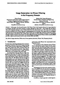
Figure 1. Flowchart of the proposed deconvolution algorithm. A fragment of House illustrates the images after each operation.
In this work we follow the above restoration scheme (regularized inversion followed by denoising) exploiting an extension of the block-matching and 3D filtering10 (BM3D). This filter is based on the assumption that there exist mutually similar patches within a natural image – the same assumption used in other non-local image filters such as.11, 12 The BM3D processes a noisy image in a sliding-window (block) manner, where block-matching is performed to find blocks similar to the currently processed one. The blocks are then stacked together to form a 3D array and the noise is attenuated by shrinkage in a 3D-transform domain. This results in a 3D array of filtered blocks. A denoised image is produced by aggregating the filtered blocks to their original locations using weighted averaging. This filter was shown10 to be highly e�ective for attenuation of additive i.i.d. Gaussian (white) noise. The contribution of this work includes • extension of the BM3D filter for additive colored noise, and • image deblurring method that exploits the extended BM3D filter for improving the regularization after regularized inversion in Fourier transform domain. The paper is organized as follows. The developed image restoration method and the extension of the BM3D filter are presented in Sections 2. Simulation results and a brief discussion are given in Section 3 and relevant conclusions are made in Section 4.
2. IMAGE RESTORATION WITH REGULARIZATION BY BM3D FILTERING The observation model given in Equation (1) can be expressed in discrete Fourier transform (DFT) domain as ] = \ Y + �˜,
(2)
where \ , Y , and �˜ are the DFT spectra of |, y, and �, respectively. Capital letters denote DFT of a signal; e.g. ] = F {}}, Y = F {y}; the only exception in that notation is for �˜ = F {�}. Due to the normalization of the
Postprint note: in Eq. (3), as in the rest of the paper, the straight vertical brackets are used for two different purposes: 1. to denote the modulus (i.e., magnitude) of a transform spectrum, as in |V|, 2. to denote the cardinality of a set, as in |X|.
forward DFT, the variance of �˜ is |[| � 2 , where |[| is the cardinality of the set [ (i.e., |[| is the number of pixels in the input image). Given the input blurred and noisy image }, the blur PSF y, and the noise variance � 2 , we apply the following two-step image deblurring algorithm, which is illustrated in Figure 1. Proposed two-step image deblurring algorithm Step 1. Regularized Inversion (RI) using BM3D with collaborative hard-thresholding. 1.1. The regularized inverse } RI is computed in DFT domain as W RI }
RI
=
Y¯ 2
|Y | + �RI |[| � 2 © ª = F �1 W RI ] ( ) © ª |Y |2 �1 = F \ + F �1 �˜W RI , 2 2 |Y | + �RI |[| �
(3)
where �RI is a regularization parameter determined empirically. Note that the obtained inverse } RI n o © ª 2 |Y | is the sum of F �1 \ |Y |2 +� , a biased estimate of |, and the colored noise F �1 �˜W RI . |[|� 2 RI
1.2. Attenuate the colored noise in } RI given by Eq. (3) using BM3D with collaborative hardthresholding (see Section 2.1); the denoised image is denoted |ˆRI . Step 2. Regularized Wiener inversion (RWI) using BM3D with collaborative Wiener filtering. 2.1. Using |ˆRI as a reference estimate, compute the regularized Wiener inverse } RW I as ¯2 ¯ ¯ ¯ Y¯ ¯\ˆ RI ¯ RW I = ¯ > W ¯ ¯ ˆ RI ¯2 ¯Y \ ¯ + �RW I |[| � 2 © ª } RW I = F �1 W RW I ] > ; < ¯ ¯ ¯ ˆ RI ¯2 A A ? @ ¯Y \ ¯ © ª RW I �1 \¯ + F �1 �˜W RW I = F } ¯2 A A ¯ ¯ = ¯Y \ˆ RI ¯ + �RW I |[| � 2 >
(4)
where, analogously to Eq. (3), �RW I is a regularization parameter and } RW I is the sum of a biased estimate of | and colored noise. 2.2. Attenuate the colored noise in } RW I using BM3D with collaborative Wiener filtering (see Section 2.2) which also uses |ˆRI as a pilot estimate. The result |ˆRW I of this denoising is the final restored image.
The BM3D filtering of the colored noise (Steps 1.2 and 2.2) plays the role of a further regularization of the sought solution. It allows the use of relatively small regularization parameters in the Fourier-domain inverses, hence reducing the bias in the estimates } RI and } RW I , which are instead essentially noisy. The BM3D denoising filter10 is originally developed for additive white Gaussian noise. Thus, to enable the attenuation of colored noise, we propose some modifications to the original filter. Before we present the extensions that enable attenuation of colored noise, we recall how the BM3D filter works; for details of the original method one can refer to.10 The BM3D processes an input image in a slidingwindow manner, where the window (block) has a fixed size Q1 × Q1 . For each processed block a 3D array is
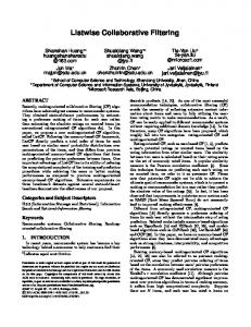
(a) BM3D with collaborative hard-thresholding
(b) BM3D with collaborative Wiener filtering Figure 2. Flowcharts of the BM3D filter extentions for colored-noise removal.
formed by stacking together blocks (from various image locations) which are similar to the current one. This process is called “grouping” and is realized by block-matching. Consequently, a separable 3D transform T3D is applied on the 3D array in such a manner that first a 2D transform, T2D , is applied on each block in the group and then a 1D transform, T1D , is applied in the third dimension. The noise is attenuated by shrinkage (e.g. hard-thresholding or empirical Wiener filtering) of the T3D -transform spectrum. Subsequently, the transform T3D is inverted and each of the filtered blocks in the group is returned to its original location. After processing the whole image, since the filtered blocks can (and usually do) mutually overlap, they are aggregated by weighted averaging to form a final denoised image. If the transforms T2D and T1D are orthonormal, the grouped blocks are non-overlapping, and the noise in the input image is i.i.d. Gaussian, then the noise in the T3D -transform domain is also i.i.d. Gaussian with the same constant variance. However, if the noise is colored as in the case of Eq. (3), then the variances � 22D (l) > for l = 1> = = = > Q12 , of the T2D -transform coe!cients are in general non constant. In the following subsections, we extend the BM3D filter to attenuate such colored noise. We note that the developed extensions are not necessarily restricted to the considered image restoration scheme but are applicable to filtering of colored noise in general. Let us introduce the notation used in what follows. With }{RI we denote a 2D block of fixed size Q1 × Q1 extracted from } RI , where { 5 [ is the coordinate of the top-left corner of the block. Let us note that this block notation is di�erent from the one (capital letter with subscript) used in10 since the capital letter in this paper is reserved for the DFT of an image. A group of collected 2D blocks is denoted by a bold-face letter with a subscript indicating the set of its grouped blocks’ coordinates: e.g., zRI V is a 3D array composed of the blocks }{RI , ;{ 5 V � [.
2.1. BM3D with collaborative hard-thresholding (Step 1.2) This filtering is applied on the noisy } RI given by Eq. (3). The variances of the coe!cients of a T2D -transform (applied to an arbitrary image block) are computed as n o°2 �2 ° ° ° RI (l) (5) � 22D (l) = °W F # T2 D ° , ;l = 1> = = = > Q12 , |[| 2
(l)
where # T2 D is the l-th basis element of T2D . The flowchart of the BM3D with collaborative hard-thresholding extended for color-noise attenuation is given in Figure 2(a). The variances � 22D are used in the block-matching to reduce the influence of noisier transform coe!cients when determining the block-distance. To accomplish this, the block-distance is computed as the c2 -norm of the di�erence between the two T2D -transformed blocks scaled by the corresponding standard deviations of the T2D -transform coe!cients. Thus, the distance is given by ° © RI ª © RI ª ° ° °2 ¡ RI RI ¢ ° �2 ° T2D }{U � T2D }{ (6) g }{U > }{ = Q1 ° ° , ° ° � 2D 2
where }{RIU is the current reference block, ©}{RI isª an arbitrary © ª block in the search neighborhood, and the operations between the three Q1 × Q1 arrays T2D }{RIU , T2D }{RI , and � 2D are elementwise. After the best-matching blocks are found (their coordinates are saved as the elements of the set V{U ) and grouped together in a 3D array, collaborative hard-thresholding is applied. It consists of applying the 3D transform T3D on the 3D group, hard-thresholding its spectrum, and then inverting the T3D . To attenuate the colored noise, the hard-threshold is made dependent on the variance of each T3D -transform coe!cient. Due to the separability of T3D , this variance depends only on the corresponding 2D coordinate within the T3D -spectrum; thus, along the third dimension of a group the variance and hence the threshold n areothe same. The hard-thresholding is performed by an elementwise with the 3D array h{U defined as multiplication of the T3D -spectrum T3D zRI V{ U
( h{U (l> m) =
¯ ¯ n o ¯ ¯ 1, if ¯T3D zRI (l> m) ¯ A �3D � 2D (l) V{U , 0, otherwise,
;l = 1> = = = > Q12 , ;m = 1> = = = > |V{U | >
where l is a spatial-coordinate index and m is an index of the coe!cients in the third dimension, �3D is a fixed threshold coe!cient and |V{U | denotes the cardinality of the set V{U . After all reference blocks are processed, the filtered blocks are aggregated by a weighted averaging, producing the denoised image |ˆRI . The weight for all filtered blocks in an arbitrary 3D group is the inverse of the sum of the variances of the non-zero transform coe!cients after hard-thresholding; for a 3D group using {U 5 [ as reference, the weight is 1 X . z{htU = h{U (l> m) � 22D (l) l=1>===>Q12 m=1>===>|V{U |
2.2. BM3D with collaborative Wiener filtering (Step 2.2) The BM3D with collaborative empirical Wiener filtering uses |ˆRI as a reference estimate of the true image |. Since the grouping by block-matching is performed on this estimate and not on the noisy image, there is no need to modify the distance calculation as in Eq. (6). The only modification from Step 2 of the original BM3D filter concerns the di�erent variances of the T3D -transform coe!cients in the empirical n oWiener filtering. This filtering RW I is performed by an elementwise multiplication of the T3D -spectrum T3D zV{ with the Wiener attenuation U coe!cients w{U defined as ¯ ¯2 n o ¯ ¯ bVRI{ (l> m)¯ ¯T3D y U w{U (l> m) = ¯ , ¯2 n o ¯ ¯ bVRI{ (l> m)¯ + � 22D (l) ¯T3D y
;l = 1> = = = > Q12 > ;m = 1> = = = > |V{U | ,
U
where, similarly to Eq. (5), the variances � 22D of the T2D -transform coe!cients are computed as � 22D (l) =
n o°2 �2 ° ° ° RW I (l) F # T2 D ° , °W |[| 2
;l = 1> = = = > Q12 .
(7)
For an arbitrary {U 5 [, the aggregation weight for its corresponding filtered 3D group is = z{wie U
X
1
w{2 U
(l> m) � 22D (l)
.
l=1>===>Q12 m=1>===>|V{U |
The flowchart of the BM3D with collaborative Wiener filtering extended for color-noise attenuation is given in Figure 2(b).
3. RESULTS AND DISCUSSION We present simulation results of the proposed algorithm, whose Matlab implementation is available online.13 All parameters, obtained after a rough empirical optimization, are fixed in all experiments (invariant of the noise variance � 2 , blur PSF y, and image |) and can be inspected from the provided implementation. In our experiments, we used the same blur PSFs and noise combinations as in.4 In particular, these PSFs are: ¢ ¡ • PSF 1: y ({1 > {2 ) = 1@ 1 + {21 + {22 > {1 > {2 = �7> = = = > 7, • PSF 2: y is a 9 × 9 uniform kernel (boxcar),
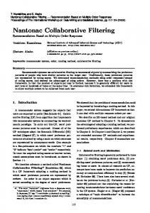
• PSF 3: y = [1 4 6 4 1]W [1 4 6 4 1] @256, • PSF 4: y is a Gaussian PSF with standard deviation 1.6, • PSF 5: y is a Gaussian PSF with standard deviation 0.4. P All PSFs are normalized so that y = 1. Table 1 presents a comparison of the improvement in signal-to-noise ratio (ISNR) for a few methods3, 4, 6, 14—16 among which are the current best.3, 4 The results of ForWaRD6 were obtained with the Matlab codes17 made available by its authors, for which we used automatically estimated regularization parameters. The results of the SA-DCT deblurring3 were produced with the Matlab implementation,18 where however we used fixed regularization parameters in all experiment in order to have fair comparison (rather than using regularization parameters dependent on the PSF and noise). The results of the GSM method19 and the SV-GSM4 are taken from.4 In most of the experiments, the proposed method outperforms the other techniques in terms of ISNR. We note that the results of the four standard experiments used in the literature (e.g.,3, 6, 7, 20 ) on image restoration are included in Table 1 as follows. • Experiment 1: PSF2, � 2 = 0=308, and Cameraman image. • Experiment 2: PSF1, � 2 = 2, and Cameraman image. • Experiment 3: PSF1, � 2 = 8, and Cameraman image. • Experiment 4: PSF3, � 2 = 49, and Lena image. The visual quality of some of the restored images can be evaluated from Figures 4, 5, and 6. One can see that fine details are well preserved and there are few artifacts in the deblurred images. In particular, ringing can be seen in some images such as the ones shown in Figure 3, where a comparison with the SA-DCT deblurring3 is made. The ringing is stronger (and ISNR is lower) in the estimate obtained by the proposed technique. We explain this as follows; let us recall that each of the noisy images } RI and } RW I (input to the extended BM3D filter) is sum of a bias and additive colored noise; the exact models of } RI and } RW I are given by Eq. (3) and (4), respectively. The ringing is part of the bias and thus it is not modeled as additive colored noise. Hence, if the ringing magnitude is relatively high, the BM3D fails to attenuate it and it is preserved in the final estimate, as in Figure 3. By comparing the results corresponding to |ˆRI and |ˆRW I in Table 2, one can see the improvement in ISNR after applying the second step (RWI using BM3D with collaborative Wiener filtering) of our two-step restoration scheme. This improvement is significant and can be explained as follows. First, the regularized Wiener inverse is more e�ective than the regularized inverse because it uses the estimated power spectrum for the inversion given
Blur: PSF2, � 2 = 0=308 (PSNR 20.76 dB)
SA-DCT deblurring3 (ISNR 8.55 dB)
Fragments of the SA-DCT result
Proposed method (ISNR 8.34 dB)
Fragments of the result by the proposed method
Figure 3. Comparison of the proposed method with the SA-DCT deconvolution method for Cameraman and PSF 2 blur kernel.
in Eq. (4). Second, the block-matching in the BM3D filtering is more accurate because it is performed within the available estimate |ˆRI rather than within the input noisy image } RW I . Third, the empirical Wiener filtering used by the BM3D in that step is more e�ective than the simple hard-thresholding used in the first step. In fact, the first step can be considered as an adaptation step that significantly improves the actual restoration performed by the second step. RW I ) the results of the naive approach of using the In Table 2, we also provide (in the row corresponding to |ˆnaive 10 original BM3D filter rather than the one extended for colored noise. This filter was applied on } RI and } RW I PQ12 2 by assuming additive i.i.d. Gaussian noise, whose variance was computed as � 2WGN = Q1�2 l=1 � 2D (l), where � 22D (·) is defined in Eq. (5) and (7) for } RI and } RW I , respectively. This variance calculation was empirically found to be better (in terms of ISNR) than estimating a noise variance from the noisy images } RI and } RW I . The benefit of using the BM3D for colored noise reaches 1 dB; in particular, the benefit is substantial for those experiments where the noise in } RI and } RW I is highly colored.
4. CONCLUSIONS The developed image deblurring method outperforms the current best techniques in most of the experiments. This performance is in line with the BM3D denoising filter10 which is among the current best denoising filters. The proposed colored-noise extension of the BM3D is not restricted to the developed deblurring method and it can in general be applied to filter colored noise. Future developments might target attenuation of ringing artifacts by exploiting the SA-DCT transform21 which, as shown in Figure 3, is e�ective in suppressing them.
Blur �2
PSF 1 2
Input PSNR ForWaRD6 GSM19 EM16 Segm.-based Reg.15 GEM14 BOA20 Anis. LPA-ICI7 SV-GSM4 SA-DCT3 Proposed
22.23 6.76 6.84 6.93 7.23 7.47 7.46 7.82 7.45 8.11 8.19
Input PSNR Segm.-based Reg.15 GEM14 BOA20 ForWaRD6 EM16 Anis. LPA-ICI7 SA-DCT3 Proposed
27.25 6.05 7.55 7.95
Input PSNR ForWaRD6 GSM19 SV-GSM4 SA-DCT3 Proposed
25.61 7.35 8.46 8.64 9.02 9.32
Input PSNR ForWaRD6 GSM19 SV-GSM4 SA-DCT3 Proposed
23.34 3.69 5.70 6.85 5.45 7.80
PSF 2 8 0=308 Cameraman 22.16 20.76 5.08 7.34 5.29 -1.61 4.88 7.59 8.04 5.17 8.10 5.24 8.16 5.98 8.29 5.55 7.33 6.33 8.55 6.40 8.34 Lena 27.04 25.84 4.90 6.97 6.10 7.79 6.53 7.97 House 25.46 24.11 6.03 9.56 6.93 -0.44 7.03 9.04 7.74 10.50 8.14 10.85 Barbara 23.25 22.49 1.87 4.02 3.28 -0.27 3.80 5.07 2.54 4.79 3.94 5.86
PSF 3 49
PSF 4 4
PSF 5 64
24.62 2.40 2.56 2.73 3.37 3.34
23.36 3.14 2.83 3.25 3.72 3.73
29.82 3.92 3.81 4.19 4.71 4.70
28.81 1.34 2.73 2.84 2.93 2.94 3.90 4.49 4.81
29.16 3.50 4.08 4.37
30.03 5.42 5.84 6.40
28.06 3.19 4.37 4.30 4.99 5.13
27.81 3.85 4.34 4.11 4.65 4.56
29.98 5.52 5.98 6.02 5.96 7.21
24.22 0.94 1.44 1.94 1.31 1.90
23.77 0.98 0.95 1.36 1.02 1.28
29.78 3.15 4.91 5.27 3.83 5.80
Table 1. Comparison of the output ISNR [dB] of a few deconvolution methods (only the rows corresponding to “Input PSNR” contain PSNR [dB] of the input blurry images).
Blur: PSF1, � 2 = 2
Output ISNR 9.32 dB
Blur: PSF1, � 2 = 8
Output ISNR 8.14 dB
Blur: PSF2, � 2 = 0=308
Output ISNR 10.85 dB
Figure 4. Deblurring results of the proposed method for House.
Blur: PSF3, �2 = 49
Output ISNR 4.81 dB
Blur: PSF4, � 2 = 4
Output ISNR 4.37 dB
Blur: PSF5, �2 = 64
Output ISNR 6.40 dB
Figure 5. Deblurring results of the proposed method for Lena.
Blur: PSF1, � 2 = 8
Output ISNR 3.94 dB
Blur: PSF2, �2 = 0=308
Output ISNR 5.86 dB
Blur: PSF3, �2 = 49
Output ISNR 1.90 dB
Figure 6. Deblurring results of the proposed method for Barbara.
Blur $ �2 $ |ˆRI |ˆRW I RW I |ˆnaive
PSF 1 2 8 7.13 5.16 8.19 6.40 7.17 6.25
PSF 2 0=308 7.52 8.34 8.14
PSF 3 49 2.31 3.34 2.57
PSF 4 4 3.23 3.73 2.71
PSF 5 64 2.46 4.70 4.63
I Table 2. ISNR comparison for: the basic estimate |ˆR I ; the final estimate |ˆRW I ; the final estimate |ˆnRW a ive obtained using the original BM3D filter instead of the one extended for colored noise. The test image was Cameraman.
REFERENCES 1. C. Vogel, Computational Methods for Inverse Problems, SIAM, 2002. 2. P. C. Hansen, Rank-Deficient and Discrete Ill-Posed Problems: Numerical Aspects of Linear Inversion, SIAM, Philadelphia, 1997. 3. A. Foi, K. Dabov, V. Katkovnik, and K. Egiazarian, “Shape-Adaptive DCT for denoising and image reconstruction,” in Proc. SPIE Electronic Imaging: Algorithms and Systems V, 6064A-18, (San Jose, CA, USA), January 2006. 4. J. A. Guerrero-Colon, L. Mancera, and J. Portilla, “Image restoration using space-variant Gaussian scale mixtures in overcomplete pyramids,” IEEE Trans. Image Process. 17, pp. 27—41, January 2007. 5. R. Neelamani, H. Choi, and R. G. Baraniuk, “Wavelet-domain regularized deconvolution for ill-conditioned systems,” in Proc. IEEE Int. Conf. Image Process., 1, pp. 204—208, (Kobe, Japan), October 1999. 6. R. Neelamani, H. Choi, and R. G. Baraniuk, “Forward: Fourier-wavelet regularized deconvolution for illconditioned systems,” IEEE Trans. Signal Process. 52, pp. 418—433, February 2004. 7. V. Katkovnik, A. Foi, K. Egiazarian, and J. Astola, “Directional varying scale approximations for anisotropic signal processing,” in Proc. European Signal Process. Conf., pp. 101—104, (Vienna, Austria), September 2004. 8. V. Katkovnik, K. Egiazarian, and J. Astola, “A spatially adaptive nonparametric regression image deblurring,” IEEE Trans. Image Process. 14, pp. 1469—1478, October 2005. 9. V. Katkovnik, K. Egiazarian, and J. Astola, Local Approximation Techniques in Signal and Image Process., vol. PM157, SPIE Press, 2006. 10. K. Dabov, A. Foi, V. Katkovnik, and K. Egiazarian, “Image denoising by sparse 3D transform-domain collaborative filtering,” IEEE Trans. Image Process. 16, pp. 2080—2095, August 2007. 11. A. Buades, B. Coll, and J. M. Morel, “A review of image denoising algorithms, with a new one,” Multiscale Modeling and Simulation 4(2), pp. 490—530, 2005. 12. C. Kervrann and J. Boulanger, “Optimal spatial adaptation for patch-based image denoising,” IEEE Trans. Image Process. 15, pp. 2866—2878, October 2006. 13. K. Dabov and A. Foi, “BM3D Filter Matlab Demo Codes.” http://www.cs.tut.fi/˜foi/GCF-BM3D. 14. J. Dias, “Fast GEM wavelet-based image deconvolution algorithm,” in Proc. IEEE Int. Conf. Image Process., 3, pp. 961—964, (Barcelona, Spain), September 2003. 15. M. Mignotte, “An adaptive segmentation-based regularization term for image restoration,” in Proc. IEEE Int. Conf. Image Process., 1, pp. 901—904, (Genova, Italy), September 2005. 16. M. A. T. Figueiredo and R. D. Nowak, “An EM algorithm for wavelet-based image restoration,” IEEE Trans. Image Process. 12, pp. 906—916, August 2003. 17. R. Neelamani, “Fourier-Wavelet Regularized Deconvolution (ForWaRD) Software for 1-D Signals and Images.” http://www.dsp.rice.edu/software/ward.shtml. 18. A. Foi and K. Dabov, “Pointwise Shape-Adaptive DCT Demobox.” http://www.cs.tut.fi/˜foi/SA-DCT. 19. J. Portilla and E. P. Simoncelli, “Image restoration using Gaussian scale mixtures in the wavelet domain,” in Proc. IEEE Int. Conf. Image Process., 2, pp. 965—968, (Barcelona, Spain), September 2003. 20. M. A. T. Figueiredo and R. Nowak, “A bound optimization approach to wavelet-based image deconvolution,” in Proc. IEEE Int. Conf. Image Process., 2, pp. 782—785, (Genova, Italy), September 2005. 21. A. Foi, V. Katkovnik, and K. Egiazarian, “Pointwise Shape-Adaptive DCT for high-quality denoising and deblocking of grayscale and color images,” IEEE Trans. Image Process. 16, pp. 1395—1411, May 2007.