Immigrant schemes for evolutionary algorithms in dynamic environments

SCIENCE CHINA April 2010 Vol. 53 No. 1: 1–11 doi:

Immigrant schemes for evolutionary algorithms in dynamic environments: Adapting the replacement rate YU Xin1 , TANG Ke1 ∗ & YAO Xin1,2 1Nature

Inspired Computation and Applications Laboratory, School of Computer Science and Technology, University of Science and Technology of China, Hefei, Anhui 230027, China, 2Centre of Excellence for Research in Computational Intelligence and Applications, School of Computer Science, University of Birmingham, Edgbaston, Birmingham B15 2TT, U.K. Received January 16, 2009; accepted April 1, 2010

Abstract One approach for evolutionary algorithms (EAs) to address dynamic optimization problems (DOPs) is to maintain diversity of the population via introducing immigrants. So far all immigrant schemes developed for EAs have used fixed replacement rates. This paper examines the impact of the replacement rate on the performance of EAs with immigrant schemes in dynamic environments, and proposes a self-adaptive mechanism for EAs with immigrant schemes to address DOPs. Our experimental study showed that the new approach could avoid the tedious work of fine-tuning the parameter and outperformed other immigrant schemes using a fixed replacement rate with traditionally suggested values in most cases. Keywords ment rate

evolutionary algorithm, dynamic optimization problem, immigrant scheme, self-adaptive replace-

Citation Yu X, Tang K, Yao X. Immigrant schemes for evolutionary algorithms in dynamic environments: Adapting the replacement rate. Sci China Inf Sci, 2010, 53: 1–11, doi:

1

Introduction

There are many challenging dynamic optimization problems (DOPs) in real-world applications. One of the best known examples is the fluctuations of the stock price over time during the process of maximizing the expected yields. Evolutionary algorithms (EAs) are good candidates for addressing DOPs since they mimic the process of natural evolution which copes very well in changing environments. However, traditional EAs tend to be easily trapped in a static environment, since the population will converge to a point of the search space, and once the environment changes, it is hard for the individuals to jump to the new promising regions of the search space. Commonly used methods to enhance the EAs’ performance in dynamic environments include re-introducing and maintaining the diversity, memory schemes and multi-population schemes [1]. While a substantial emphasis has been put on the continuous domain, Rohlfshagen and Yao [2] recently analyzed dynamics in the combinatorial domain via an example of the subset sum problem. They showed that some assumptions traditionally regarded as being reasonable for developing new algorithms did not necessarily hold in the case of discrete optimization. ∗ Corresponding

author (email: [email protected])

2

Yu X, et al.

Among approaches for DOPs, immigrant schemes have proved to be effective via maintaining the diversity of the population throughout the run [3 − 7]. They work by replacing a predefined proportion of the population with the newly generated immigrants at the end of each generation. When designing an immigrant scheme, generally there are four issues needing to be addressed, namely the mechanism of generating immigrants, the replacement strategy, the survival capability of the introduced immigrants in the population, and the replacement rate [3]. Over the years, researchers have already done some research on the first three issues, e.g., refs. [4, 5, 6] for the mechanism of generating immigrants, ref. [7] for the replacement strategy and the survival capability of the new immigrants in the population, whereas there has been little work on the replacement rate. The replacement rate represents the proportion of the population that will be replaced by immigrants. All previously designed immigrant schemes simply set the replacement rate to a fixed value, e.g., 0.2 [4, 5] or 0.3 [6]. In this paper, the impact of the replacement rate on the performance of EAs with immigrant schemes in dynamic environments is examined, and a self-adaptive scheme is designed for immigrant schemes. It is known that the self-adaptation has been widely and successfully applied to the field of evolutionary computation (EC) [8], such as genetic algorithms (GAs) [9, 10, 11], evolutionary programming (EP) [12], evolution strategy (ES) [13], differential evolution (DE) [14], and particle swarm optimization (PSO) [15]. However, these attempts all aimed at optimization problems in stationary environments. The main contributions of this paper are listed as follows. First, we fill the gap of research on the replacement rate for immigrant schemes. Second, we eliminate the parameter replacement rate. Although we introduce a new parameter, experimental results showed that the performance of the algorithm was much less sensitive to the new parameter than to the replacement rate. Third, the performance when using the self-adaptive mechanism outperformed that when traditionally suggested values (i.e., 0.2 and 0.3) of the replacement rate were used in most cases. Furthermore, the self-adaptation avoids fine-tuning the parameter replacement rate to achieve the best performance in different kinds of environment. There is only a slight degradation in the performance. The rest of this paper is organized as follows: Section 2 briefly reviews immigrant schemes for EAs in dynamic environments. Section 3 presents the self-adaptive replacement rate for immigrant scheme. Section 4 describes the experimental setup for this study. The experimental results and analysis are presented in Section 5. Finally, conclusions are drawn in Section 6.

2

Immigrant schemes for DOPs

Classic EAs tend to converge to a single solution, and when the environment changes, it takes some time for the population to adapt to the new environment and move towards the new promising region, because nearly all the individuals of the population concentrate on a point of the search space. To address this problem, immigrant schemes are introduced into EAs to maintain the diversity of the population throughout the run [3 − 7, 16 − 18]. They work by replacing a predefined proportion of the population with newly generated immigrants at the end of each generation. The most prominent approach to generate immigrants seems to create immigrants randomly. Grefenstette [16] used randomly generated individuals to replace the worst individuals of the population in each generation. The random immigrant scheme works on the analogy of the flux of immigrants that wander in and out of a population between two generations in nature [17]. His study shows that the random immigrant scheme works well in environments where there are occasional, large changes in the location of the optimum. Branke [19] stated that continuous adaptation only made sense when problems to be studied featured “small to medium” environmental changes, otherwise to restart the search from scratch would be the proper choice. Under this assumption, compared with randomly generating immigrants, it would be more suitable to generate immigrants based on the information of the population, since individuals in the previous environment may still be quite fit in the new environment. According to the way in which the information of the population is used, existing immigrant schemes

Yu X, et al.

Sci China Inf Sci

April 2010 Vol. 53 No. 1

3

are categorized into the direct immigrant scheme and the indirect immigrant scheme, respectively [3]. The direct immigrant scheme generates immigrants based on the current population. On the other hand, the indirect immigrant scheme first builds a model based on the current population, then generates immigrants according to the model. Examples of the direct immigrant scheme include the elitism-based immigrant scheme [5] in which immigrants come from mutating the elite from previous generation, and a hybrid immigrant scheme combing the elitism-based, the traditional random, and the dualism-based immigrant schemes for GAs to deal with DOPs [6]. The former scheme aims at improving the performance on GAs in slowly and slightly changing environments while the latter scheme makes GAs adapted to more severely changing environments. As examples of the indirect immigrant scheme, Yang [18] used a memory as the model to generate immigrants. Besides, in ref. [4], a vector with the allele distribution of the population was first calculated and then was used to generate immigrants. Moreover, experiments were done to thoroughly investigate the difference in the behaviors of different types of immigrant schemes and to compare their performance in dynamic environments [3]. The authors also proposed a hybrid immigrant scheme which combined the merits of the two types of immigrant schemes.

3

Adapting the replacement rate

The replacement rate was claimed to be an important issue needed to be considered when designing immigrant schemes for EAs in dynamic environments [3]. Grefenstette [16] conducted an experiment showing that for the non-stationary test function in his study, random immigrant schemes for GAs using a replacement rate 0.3 exhibited the best off-line performance. After that, all the immigrant schemes developed so far adopted 0.2 or 0.3 as the fixed replacement rate throughout the run [3 − 6, 16]. However, we believe that a fixed replacement rate is not the best choice, since for different immigrant schemes, at different stages of evolutionary process, and under different environments, the most appropriate replacement rate varies. It is natural that the replacement rate should be set to a proper value such that a good balance between exploration and exploitation can be kept. If the immigrant scheme has a positive effect, i.e., the introduced immigrants can help the population to move to the new optimum when an environmental change occurs, or can speed up the convergence of the population when there is no change, the replacement rate should be enlarged. Otherwise, to prevent the searching process of EAs from being disrupted, the replacement rate should be reduced. In order to adapt the value of the replacement rate during the searching process, we must estimate the effect of the current immigrant scheme. If the current immigrant scheme has a positive effect, more immigrants are encouraged to be introduced, i.e., the value of the replacement rate should be enlarged. Otherwise, the value of the replacement rate should be reduced. We propose to monitor the effect of an immigrant scheme as below. 3.1

Evaluating the effect of immigrant schemes

Denote the number of immigrants at time 𝑡 by 𝑁 𝐼𝑚(𝑡), the fitness value of the 𝑖th immigrant at time 𝑡 by 𝑓𝑖𝑚𝑖 (𝑡) (𝑖 = 1, 2, . . . , 𝑁 𝐼𝑚(𝑡)), the median fitness value of the population at time 𝑡 by 𝑓𝑚𝑒𝑑𝑖𝑎𝑛 (𝑡), and the number of immigrants satisfying the condition 𝑓𝑖𝑚𝑖 (𝑡) ⩾ 𝑓𝑚𝑒𝑑𝑖𝑎𝑛 (𝑡) at time 𝑡 by 𝑁 𝐼𝑚(𝑡){𝑓𝑖𝑚𝑖 (𝑡) ⩾ 𝑓𝑚𝑒𝑑𝑖𝑎𝑛 (𝑡)}. Then the effect of an immigrant scheme at time 𝑡 is denoted by 𝐸𝑓 𝑓 (𝑡) and can be evaluated as follows: 𝑁 𝐼𝑚(𝑡){𝑓𝑖𝑚𝑖 (𝑡) ⩾ 𝑓𝑚𝑒𝑑𝑖𝑎𝑛 (𝑡)} 𝐸𝑓 𝑓 (𝑡) = . (1) 𝑁 𝐼𝑚(𝑡) Given a predefined threshold 𝛿𝑒𝑓 𝑓 , the immigrant scheme can be regarded as having a positive effect at time 𝑡 if 𝐸𝑓 𝑓 (𝑡) > 𝛿𝑒𝑓 𝑓 . Note that in this paper, the time 𝑡 is measured in generations. Instead of the median fitness value of the population used in Eq. (1), the best or the worst fitness values of the population can also be used. We choose “median” because it is not too extreme. It can be seen from the Eq. (1) that we first count the number of immigrants that are regarded as being fit according to the results of comparing with a certain criterion derived from the current population, and then we can measure the effect of an immigrant scheme by calculating the proportion of the obtained

4

Yu X, et al.

number in the whole population of the immigrants. Naturally, this measure is by no means the most objective, but it can to some extent reflect the effect of the immigrant scheme. Therefore, we design this measure for the self-adaptive scheme described below. 3.2

Adapting the replacement rate

As mentioned above, if the current immigrant scheme has a positive effect, the replacement rate should be increased, and otherwise it should be decreased. Therefore, the replacement rate at time 𝑡 (denoted by 𝑅(𝑡)) can be derived from 𝑅(𝑡 − 1) according to the effect of the immigrant scheme at time 𝑡 − 1. Given the effect of immigrant scheme at time 𝑡 − 1, we have the following replacement rate updating rule: ⎧   ⎨ 𝑅(𝑡 − 1) + 0.1, if 𝐸𝑓 𝑓 (𝑡 − 1) > 𝛿𝑒𝑓 𝑓 𝑅(𝑡) = (2) 𝑅(𝑡 − 1) − 0.1, if 𝐸𝑓 𝑓 (𝑡 − 1) < 𝛿𝑒𝑓 𝑓   ⎩ 𝑅(𝑡 − 1), otherwise. 𝑅(𝑡) is bounded in the interval (0, 1), and 𝑅(0) = 0.5. It can be seen that our approach introduces a new parameter 𝛿𝑒𝑓 𝑓 . However, we will show that the performance is much less sensitive to the value of 𝛿𝑒𝑓 𝑓 than to the replacement rate as in the immigrant scheme without the adaptation mechanism. 3.3

Time complexity of the adaptation mechanism

The additional cost added by the adaptation process is determined by the calculation of 𝐸𝑓 𝑓 (𝑡) in Eq. (1) and the update of 𝑅(𝑡) in Eq. (2). When computing the runtime complexity, since data transfer operations like copy/assignment, etc. hardly require any complex digital circuitry like adder, comparator, etc. [20, 21], we only consider the fundamental floating-point arithmetic and logical operations performed by the adaptation mechanism. Given the population of size 𝑁 and at time 𝑡, the complexity 𝑇 (𝑁 ) of the adaptation consists of finding the median of the population, calculating 𝐸𝑓 𝑓 (𝑡 − 1), and updating 𝑅(𝑡). Based on the partition algorithm similar to the one used in quicksort, finding the median needs 𝑂(𝑁 ) comparisons on average and 𝑂(𝑁 2 ) comparisons in the worst case [20]. Calculating 𝐸𝑓 𝑓 (𝑡 − 1) needs 𝑅(𝑡 − 1) ⋅ 𝑁 comparisons, and updating 𝑅(𝑡) needs one comparison and one arithmetic operation (when 𝐸𝑓 𝑓 (𝑡) ∕= 𝛿𝑒𝑓 𝑓 ). Therefore, the time complexity of the adaptation mechanism 𝑇 (𝑁 ) = 𝑂(𝑁 ) on average and 𝑇 (𝑁 ) = 𝑂(𝑁 2 ) in the worst case. In real-world applications, the evaluation of an individual may consume too much time. Therefore, given a population of size 𝑁 , in one generation, compared with 𝑁 times of evaluation, the time consumed by floating-point arithmetic and logical operations introduced by the adaptation process is negligible.

4 4.1

Experimental design Dynamic test environments

Using the DOP generator proposed in refs. [22, 23], dynamic environments can be constructed from any binary-encoded stationary function 𝑓 (𝒙) (𝒙 ∈ {0, 1}𝑙) by a bitwise exclusive-or (XOR) operator. The generator basically works as follows: The operation 𝒙 ⊕ 𝑴 is performed before evaluation of the individual 𝒙 in the population, where ⊕ is the XOR operator (i.e., 1 ⊕ 1 = 0, 1 ⊕ 0 = 1, 0 ⊕ 0 = 0) and 𝑴 is a previously created binary mask. Then the resulting individual is evaluated. When there is a change at generation 𝑡, we have 𝑓 (𝒙, 𝑡 + 1) = 𝑓 (𝒙 ⊕ 𝑴 , 𝑡). With this DOP generator, the speed and the severity of the environmental changes are controlled by parameters 𝜏 and 𝜌 ∈ (0.0, 1.0) respectively. The parameter 𝜏 is the number of generations between two changes, and the parameter 𝜌 is the ratio of ones in an intermediate binary template that is created for each environment and used to generate the mask 𝑴 . Smaller 𝜏 means faster changes while bigger 𝜌 indicates severer changes. More details about the DOP generator can be found in refs. [22, 23]. In this paper, dynamic test environments are systematically constructed from a stationary problems, i.e., the OneMax problem, via the DOP generator with 𝜏 set to 10, 50, and 100 and 𝜌 set to 0.05, 0.5,

Yu X, et al.

Sci China Inf Sci

April 2010 Vol. 53 No. 1

5

and 0.9 respectively. In all, a series of 9 DOPs are generated. The indices of the environment used in the experiment are shown in Table 1. Table 1 Environmental indices used in the experiment Environmental Parameters 𝜏 = 10 𝜏 = 50 𝜏 = 100 𝜌 = 0.1 1 2 3 𝜌 = 0.5 4 5 6 𝜌 = 0.9 7 8 9

4.1.1

The OneMax problem

The OneMax problem has only one optimum and aims to maximize the number of ones in a binary string. So the fitness of an individual is the number of ones in the binary string. Given a binary string 𝒙 of length 𝐿, the problem is defined as follows: maximize 𝑓 (𝒙) =

𝐿 ∑

𝑥𝑖 ,

(3)

𝑖=1

where 𝑓 (𝒙) is the fitness of a binary string 𝒙 = (𝑥1 , . . . , 𝑥𝐿 ) ∈ 𝐼 = {0, 1}𝐿. In our experiment we set the length of the binary string 𝐿 to 100. 4.1.2

The Royal Road problem

The Royal Road function is a binary problem with only one optimum and many large plateaus. The function used in this paper is similar to the Royal Road function introduced in ref. [24]. It is defined on a 100-bit binary string that consists of 25 contiguous building blocks, each of which is 4-bit long and contributes 𝑐𝑖 = 4 (𝑖 = 1, . . . , 25) to the total fitness if and only if every bit is one. Therefore, the fitness of a string 𝒙 is the sum of the coefficients 𝑐𝑖 corresponding to each given schema 𝑠𝑖 , of which 𝒙 ∈ 𝑠𝑖 , i.e.: maximize 𝑓 (𝒙) =

25 ∑

𝑐𝑖 𝛿𝑖 (𝒙),

(4)

𝑖=1

where 𝛿𝑖 (𝒙) = 4.2

{

1, 0,

if 𝒙 ∈ 𝑠𝑖 otherwise.

(5)

Experimental setup

In order to investigate the efficacy of the proposed self-adaptive mechanism for immigrant schemes, we applied it to two previously proposed immigrant schemes for GAs, i.e., the random immigrant scheme GA (RIGA) [16] and the elitism-based immigrant scheme GA (EIGA) [5]. In each generation, RIGA generates immigrants randomly, and EIGA generates immigrants by mutating the elite of the population at previous generation. These immigrant schemes with self-adaptive replacement rates are denoted by SRRIGA and SREIGA (“SR” stands for “self-adaptive rate”), respectively in this paper. RIGA and SRRIGA are the same except that the former has a fixed replacement rate while the latter has the selfadaptive replacement rate. The same relation exists between EIGA and SREIGA. The pseudo-codes of the algorithms are given in Table 2, where 𝑝𝑐 is the crossover probability, 𝑝𝑚 is the mutation probability, and 𝑝𝑚 𝑒𝑖 is the probability of mutating the elite, and 𝑛 is the population size. The algorithms’ genetic operations and parameters were set as follows: generational, uniform crossover with crossover probability 𝑝𝑐 = 0.6, bit-flipping mutation with mutation rate 𝑝𝑚 = 0.01, fitness proportional selection implemented via stochastic universal sampling algorithm with elitism of size 1, chromosome length 𝐿 = 100, and population size 𝑛 = 100. For EIGA, 𝑝𝑚 𝑒𝑖 was set to 0.01. For RIGA and EIGA, in order to study the impact of replacement rate on the performance of them in dynamic environments, for each algorithm the replacement rate was set from 0.1 to 0.9 with step 0.1. For SRRIGA and SREIGA, to investigate the impact of 𝛿𝑒𝑓 𝑓 on the performance of algorithms, for each algorithm the value 𝛿𝑒𝑓 𝑓 was set from 0.1 to 0.9 with step 0.1.

6

Yu X, et al.

Table 2

Pseudo-code for GAs with random immigrants (RIGA), with elitism-based immigrants (EIGA), and their self-adaptive variants (SRRIGA and SREIGA) 1: begin 2: 𝑡 := 0 and initialize population 𝑃 (0) randomly 3: evaluate population 𝑃 (0) 4: if self-adaptation is used then // for SRRIGA and SREIGA 5: 𝑅(0) := 0.5 6: else 7: set 𝑅(0) to a predefined value 8: end if 9: repeat 10: 𝑃 ′ (𝑡) := selectForReproduction(𝑃 (𝑡)) 11: crossover(𝑃 ′ (𝑡),𝑝𝑐 ) // 𝑝𝑐 is the crossover probability 12: mutate(𝑃 ′ (𝑡),𝑝𝑚 ) // 𝑝𝑚 is the mutation probability 13: evaluate population 𝑃 ′ (𝑡) 14: 15: 16: 17: 18: 19: 20: 21: 22: 23: 24: 25: 26:

if random immigrant scheme is used then // for RIGA generate 𝑅(𝑡) × 𝑛 random immigrants evaluate these random immigrants end if if elitism-based immigrant scheme is used then // for EIGA denote the elite in 𝑃 (𝑡 − 1) by 𝐸(𝑡 − 1) generate 𝑅(𝑡) × 𝑛 immigrants by mutating 𝐸(𝑡 − 1) with 𝑝𝑚 𝑒𝑖 evaluate these elitism-based immigrants end if if self-adaptation is used then // for SRRIGA and SREIGA calculate Eff(t) according to Eq. (1) update R(t) according to Eq. (2) end if

replace the worst individuals in 𝑃 ′ (𝑡) with the generated immigrants 28: 𝑃 (𝑡 + 1) := 𝑃 ′ (𝑡) 29: until the termination condition is met 30: end 27:

For each algorithm on a DOP, 30 independent runs were executed with the same set of random seeds, and for each run, 50 environmental changes were allowed. The off-line performance used to compare the algorithms was defined as below: 𝐹 𝐵𝑂𝐺 =

𝐺 𝑁 1 ∑ 1 ∑ ( 𝐹𝐵𝑂𝐺𝑖𝑗 ), 𝐺 𝑖=1 𝑁 𝑗=1

(6)

where 𝐺 is the number of generations for a run, 𝑁 is the number of runs, and 𝐹𝐵𝑂𝐺𝑖𝑗 is the best-ofgeneration fitness of generation 𝑖 of run 𝑗. In the experiments, we would like to investigate the impact of the replacement rate on the performance of algorithms, the impact of the newly introduced parameter 𝛿𝑒𝑓 𝑓 on the performance of algorithms, and compare the performance of algorithms with and without the adaptation. The results and the related analyses are shown in the next section.

5 5.1

Experimental results The impact of replacement rate on the performance of algorithms

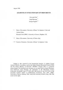
The off-line performance of RIGA and EIGA on all DOPs against the replacement rate is plotted in Figure 1. From Figure 1, it can be seen that for RIGA on the OneMax problem, when the environment changes slightly, i.e., 𝜌 = 0.1, smaller replacement rates always show higher performance than larger replacement rates. This is because when the environment changes slightly, the individuals in the population are still quite fit in the new environment, and the introduced randomly created individuals will disrupt the ongoing searching process, leading to the degradation in the performance. Besides, for other kinds of

Yu X, et al.

RIGA, OneMax

RIGA, RoyalRoad

75

70

65

100

95

90

80

ρ=0.1 τ=10 ρ=0.5 τ=10 ρ=0.9 τ=10 ρ=0.1 τ=50 ρ=0.5 τ=50 ρ=0.9 τ=50 ρ=0.1 τ=100 ρ=0.5 τ=100 ρ=0.9 τ=100

70 60 50 40 30

60 0.1

0.2

0.3

0.4

0.5

0.6

0.7

Replacement Rate

0.8

0.9

EIGA, RoyalRoad

100

90

20 0.1

90

ρ=0.1 τ=10 ρ=0.5 τ=10 ρ=0.9 τ=10 ρ=0.1 τ=50 ρ=0.5 τ=50 ρ=0.9 τ=50 ρ=0.1 τ=100 ρ=0.5 τ=100 ρ=0.9 τ=100

85 80 75 70 65

0.3

0.4

0.5

0.6

0.7

Replacement Rate

0.8

0.9

55 0.1

80

ρ=0.1 τ=10 ρ=0.5 τ=10 ρ=0.9 τ=10 ρ=0.1 τ=50 ρ=0.5 τ=50 ρ=0.9 τ=50 ρ=0.1 τ=100 ρ=0.5 τ=100 ρ=0.9 τ=100

70 60 50 40 30

60 0.2

Offline Performance

ρ=0.1 τ=10 ρ=0.5 τ=10 ρ=0.9 τ=10 ρ=0.1 τ=50 ρ=0.5 τ=50 ρ=0.9 τ=50 ρ=0.1 τ=100 ρ=0.5 τ=100 ρ=0.9 τ=100

80

EIGA, OneMax

100

Offline Performance

85

Offline Performance

Offline Performance

90

7

April 2010 Vol. 53 No. 1

Sci China Inf Sci

0.2

0.3

0.4

0.5

0.6

0.7

Replacement Rate

0.8

0.9

20 0.1

0.2

0.3

0.4

0.5

0.6

0.7

0.8

0.9

Replacement Rate

Figure 1 The impact of the replacement rate on the performance of algorithms in dynamic environments. environments on the OneMax problem, i.e., 𝜌 = 0.5 and 𝜌 = 0.9, and all kinds of environments except 𝜌 = 0.5, 0.9 and 𝜏 = 10 on the Royal Road problem, the performance first increases and then decreases as the value of replacement rate increases. The reason is that these kinds of environments are characterized as more severe degree of changes, so neither must the value of replacement rate be too small in order to help the population to jump out of the old promising region, nor must the value of replacement rate be too large in order to protect the searching process from being disrupted. For EIGA, it can be seen from Figure 1 that on the OneMax problem, except when 𝜏 = 10 and 𝜌 = 0.5, 0.9, larger replacement rates always exhibit higher performance than smaller replacement rates. This is because EIGA is especially designed for addressing slightly and slowly changing environments. When the environment changes slightly, i.e., 𝜌 = 0.1, since the new optimum is not far from the old one, elitism-based immigrants can be quite fit in the new environment. On the other hand, when the environment changes slowly, i.e., 𝜏 = 50 and 100, there is enough time for the population to recover from the last change of the environment, and to find the new optimum quickly with the help of elitism-based immigrants even when the environment changes significantly (i.e., 𝜌 = 0.9). However, when the environment changes rapidly, i.e., 𝜏 = 10, there is no time for the population to quickly recover under more severe changes (i.e., 𝜌 = 0.5 and 0.9). Therefore, increasing the value of replacement rate does not improve the performance under this situation. In addition, on the Royal Road problem, increasing the replacement rate brings a little performance enhancement for most slightly and slowly changing environments, and sometimes there is even a little degradation in the performance. This is because by mutating the elite, some good building blocks may be destroyed. In summary, the experimental results validate our claim in Section 3 that for different immigrant schemes, at different stages of evolutionary process, and under different environments, there exist different replacement rates to maximize the performance. 5.2

The impact of 𝛿𝑒𝑓 𝑓 on the performance of algorithms

The off-line performance of SRRIGA and SREIGA on all DOPs against the value of 𝛿𝑒𝑓 𝑓 is plotted in Figure 2. From this figure, several results can be observed and analyzed as follows. First, it can be seen from Figure 2 that on the OneMax problem, when the environment changes slightly (i.e., 𝜌 = 0.1) or slowly (i.e., 𝜏 = 50 and 100), the performance of SRRIGA increases while 𝛿𝑒𝑓 𝑓 increases from 0.1 to 0.3, and then maintains nearly the same level when 𝛿𝑒𝑓 𝑓 is equal to or larger than 0.3. On the other hand, when the environment changes both significantly and rapidly, the performance of SRRIGA keeps a certain level when 𝛿𝑒𝑓 𝑓 is not larger than 0.2 and decreases otherwise. This can be explained as follows. Through the definition of 𝐸𝑓 𝑓 (𝑡) in Eq. (1) and the meaning of 𝛿𝑒𝑓 𝑓 , we know that if 𝛿𝑒𝑓 𝑓 is too small, the introduced immigrants will easily tend to be regarded as having a positive effect, and thus according to Eq. (2), the value of replacement rate will increase. On the other hand, if 𝛿𝑒𝑓 𝑓 is too large, the immigrants introduced will mostly be regarded as having a negative effect, causing the reduction of the value of replacement rate. Meanwhile, from subsection 5.1, we know that immigrants in SRRIGA are useful for rapidly and significantly changing environments, and are harmful for other kinds of environments if their number is too large. Therefore, in slightly or slowly changing environments, the performance when

8

Yu X, et al.

SRRIGA, OneMax

SRRIGA, RoyalRoad

75

70

65

60 0.1

100

95

90

ρ=0.1 τ=10 ρ=0.5 τ=10 ρ=0.9 τ=10 ρ=0.1 τ=50 ρ=0.5 τ=50 ρ=0.9 τ=50 ρ=0.1 τ=100 ρ=0.5 τ=100 ρ=0.9 τ=100

70 60 50 40 30

0.2

0.3

0.4

0.5

δeff

0.6

0.7

0.8

20 0.1

0.9

SREIGA, RoyalRoad

100

80

90

ρ=0.1 τ=10 ρ=0.5 τ=10 ρ=0.9 τ=10 ρ=0.1 τ=50 ρ=0.5 τ=50 ρ=0.9 τ=50 ρ=0.1 τ=100 ρ=0.5 τ=100 ρ=0.9 τ=100

85 80 75 70 65

Offline Performance

ρ=0.1 τ=10 ρ=0.5 τ=10 ρ=0.9 τ=10 ρ=0.1 τ=50 ρ=0.5 τ=50 ρ=0.9 τ=50 ρ=0.1 τ=100 ρ=0.5 τ=100 ρ=0.9 τ=100

80

SREIGA, OneMax

90

Offline Performance

85

Offline Performance

Offline Performance

90

0.3

0.4

0.5

δeff

0.6

0.7

0.8

55 0.1

0.9

ρ=0.1 τ=10 ρ=0.5 τ=10 ρ=0.9 τ=10 ρ=0.1 τ=50 ρ=0.5 τ=50 ρ=0.9 τ=50 ρ=0.1 τ=100 ρ=0.5 τ=100 ρ=0.9 τ=100

70 60 50 40 30

60

0.2

80

0.2

0.3

0.4

0.5

δeff

0.6

0.7

0.8

20 0.1

0.9

0.2

0.3

0.4

0.5

δeff

0.6

0.7

0.8

0.9

Figure 2 The impact of the value of 𝛿𝑒𝑓 𝑓 on the performance of algorithms in dynamic environments.

SRRIGA, RoyalRoad, τ=50, ρ=0.5

65 60

100

200

300

400

70 60 50 40 30 20 10 0

500

200

300

400

Generation

Generation

SRRIGA, OneMax, τ=50, ρ=0.5

SRRIGA, RoyalRoad, τ=50, ρ=0.5 0.7

0.6

0.6

0.5

0.5

0.4

0.4

0.3

0.2

0.1

0.1

100

200

300

Generation

400

500

0 0

90 85 80 75 70 65 60 55 100

200

300

400

200

300

Generation

60 50 40 30 20 10 0 0

500

100

SREIGA, OneMax, τ=50, ρ=0.5

400

500

300

400

500

SREIGA, RoyalRoad, τ=50, ρ=0.5

1

1

0.95

0.95

0.9

0.9

0.85

0.85 0.8

0.75

0.75

0.7

0.7

0.65

0.65

0.6

0.6

0.55

0.55

0.5 0

200

Generation

0.8

100

70

Generation

0.3

0.2

95

50 0

500

R(t)

0.7

0 0

100

Best−Of−Generation Fitness

70

80

100

Best−Of−Generation Fitness

75

55 0

R(t)

Best−Of−Generation Fitness

80

R(t)

Best−Of−Generation Fitness

85

SREIGA, RoyalRoad, τ=50, ρ=0.5

SREIGA, OneMax, τ=50, ρ=0.5

80

R(t)

SRRIGA, OneMax, τ=50, ρ=0.5 90

100

200

300

Generation

400

500

0.5 0

100

200

300

400

500

Generation

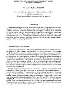
Figure 3 The dynamics of the maximal fitness and the replacement rate of a run (𝛿 = 0.3) in the first 10 environments (𝜏 = 50 and 𝜌 = 0.5).

𝛿𝑒𝑓 𝑓 is too small (e.g., 𝛿𝑒𝑓 𝑓 = 0.1) is worse than the performance when 𝛿𝑒𝑓 𝑓 is larger (e.g., 𝛿𝑒𝑓 𝑓 ⩾ 0.3), while in significantly and rapidly changing environments, the performance will degrade when 𝛿𝑒𝑓 𝑓 > 0.2. Second, the performance of SRRIGA on the Royal Road problem generally does not rely on 𝛿𝑒𝑓 𝑓 , which is due to the fact that random immigrants may introduce useful schemata, and at the same time the harmful schemata which can break good building blocks via crossover. On the other hand, the performance of SREIGA on both problems is generally insensitive to 𝛿𝑒𝑓 𝑓 . This is because immigrants in SREIGA are always useful in a stationary period between two consecutive changes since they can speed up the convergence rate. Therefore, no matter how much 𝛿𝑒𝑓 𝑓 is, immigrants in SREIGA will have a positive effect in most time, see Figure 3. Moreover, from Figure 3, on the OneMax problem, we can see that the replacement rate increased after the environmental changes, which indicates that the random immigrants at that time were useful for the population to move to the new optimum, and then the it decreased which means the promising area was found and too many immigrants could disrupt the ongoing search. To sum up, the performance of the algorithm with adaptation of the replacement rate is not so sensitive to 𝛿𝑒𝑓 𝑓 as that of the algorithm without adaptation to the value of the replacement rate. More importantly, there exist some values of 𝛿𝑒𝑓 𝑓 (e.g., 𝛿𝑒𝑓 𝑓 ∈ [0.3, 0.9]) that can yield satisfying performance for every immigrant scheme in different kinds of environments experimented. Therefore, the tedious work of fine-tuning the value of replacement rate in algorithms without adaptation in order to maximize the performance for a certain immigrant scheme and for a certain environment can be avoided.

Yu X, et al.

Comparing RIGA variants, Royal Road

80

75

70

80 70 60 50 40 30

65 1

2

3

4

5

6

7

Environmental Index

8

9

20 1

100 EIGA 0.2 EIGA 0.3 SREIGA

95

Offline Performance

85

Comparing EIGA variants, Royal Road

100 RIGA 0.2 RIGA 0.3 SRRIGA

90

Offline Performance

Offline Performance

Comparing EIGA variants, OneMax

100

RIGA 0.2 RIGA 0.3 SRRIGA

90 85 80 75 70 65

3

4

5

6

7

Environmental Index

8

9

55 1

80 70 60 50 40 30

60 2

EIGA 0.2 EIGA 0.3 SREIGA

90

Offline Performance

Comparing RIGA variants, OneMax 90

9

April 2010 Vol. 53 No. 1

Sci China Inf Sci

2

3

4

5

6

7

Environmental Index

8

9

20 1

2

3

4

5

6

7

8

9

Environmental Index

Figure 4 Comparison between immigrant schemes with and without adaptation mechanism. 5.3

Adaptation versus no adaptation

The experimental results regarding overall performance are presented in Table 3, where the performance of the algorithm adopting adaptation scheme when 𝛿𝑒𝑓 𝑓 = 0.3 is compared with the performance of the algorithm with a fixed replacement rate. We did experiments with the replacement rate being from 0.1 to 0.9 with step size 0.1. Here, only the results obtained with the commonly used values 0.2 and 0.3 for the fixed replacement rate scheme are presented in Table 3. The results are also given in Figure 4. Furthermore, the best results achieved with the fixed replacement rate are also presented, together with the corresponding replacement rate (the column “𝑏𝑒𝑠𝑡(𝑅)”). These three sets of results were compared to the results obtained by the self-adaptive replacement rate. Wilcoxon rank sum tests at a 0.05 level of significance were used to check whether there existed significant difference between fixed and self-adaptive replacement rates. The results of statistical tests are also presented in Table 3, where the result is marked as “+” or “−” when the algorithm with adaptation scheme (𝛿𝑒𝑓 𝑓 = 0.3) is significantly better or worse than the algorithm without adaptation scheme, respectively, and “∼” indicates there is no statistical difference between two algorithms. Analyzing the results in Table 3 and Figure 4, several phenomena can be observed and can be explained as below. First, comparing the self-adaptive rate with commonly used replacement rates, we can see that on the OneMax problem applying adaptation to EIGA improves its performance a lot except when 𝜌 = 0.9 and 𝜏 = 10. This is because when the environment changes both severely and rapidly, immigrants generated via mutating the elite from previous generation usually have low fitness in the new environment. For RIGA on the other hand, the difference between the performance of the algorithm before and after using the adaptation scheme is not so obvious. A probable reason is that the stochasticity in RIGA can sometimes mislead the adaptation of the replacement rate. On the Royal Road problem, due to the reason described in subsection 5.2, the performance enhancement of SREIGA is not obvious, and the performance of SRRIGA is the worst. Second, comparing the performance using self-adaptive rate with the best results obtained using fixed replacement rate (the column “𝑏𝑒𝑠𝑡(𝑅)”), the former is beaten by the latter in most cases. This can be expected since the results shown in the column “𝑏𝑒𝑠𝑡(𝑅)” are obtained via fine-tuning the replacement rate. Fortunately, except for SRRIGA on the Royal Road problem, even if the algorithm with adaptation when 𝛿𝑒𝑓 𝑓 = 0.3 does not show the best score, its performance level is still quite satisfactory. Considering the tedious work of fine-tuning the replacement rate for every immigrant scheme and for every environment, it is worthy using our adaptation scheme and setting the value of 𝛿𝑒𝑓 𝑓 simply to 0.3. The very slight performance degradation when using the adaptive scheme is more than compensated for by the convenience of not having to set the replacement rate by hand.

6

Conclusions

This paper examined the impact of the replacement rate on the performance of EAs with immigrants schemes in dynamic environments. A self-adaptive replacement rate was proposed to address DOPs. Experimental studies were carried out on a series of dynamic problems to investigate the efficacy of our approach. From the obtained results several conclusions can be drawn: First, the replacement rate is an

10

Yu X, et al.

important issue when designing immigrant schemes for EAs to cope with DOPs, and the most appropriate choice of the replacement rate varies according to the problems being solved, environments encountered, mechanisms used to generate immigrants, and stages at which the search is going. Second, comparing with immigrant schemes with a fixed replacement rate adopting traditionally used values (i.e., 0.2 and 0.3), our proposed adaptation scheme can promote the performance of immigrants schemes in most cases. Finally, compared with tedious work of fine-tuning the replacement rate manually, the proposed approach is more convenient and can produce sufficiently good solutions under different conditions. However, to pay a price for this convenience, the performance decreases a little in some cases. As to the future work, some other ways of adapting the replacement rate are under investigation. Table 3

Experimental results regarding overall performance and results of comparing the performance of algorithms via

statistical tests Adaptation vs OneMax Results Royal Road Results No Adaptation Overall performance Statistical test results Overall performance Statistical test results GAs and Parameters 0.2 0.3 𝛿𝑒𝑓 𝑓 = 0.3 𝑏𝑒𝑠𝑡(𝑅) vs 0.2 vs 0.3 vs 𝑏𝑒𝑠𝑡(𝑅) 0.2 0.3 𝛿𝑒𝑓 𝑓 = 0.3 𝑏𝑒𝑠𝑡(𝑅) vs 0.2 vs 0.3 vs 𝑏𝑒𝑠𝑡(𝑅) 𝜏 = 10 RIGA 75.69 75.11 75.83 75.93(0.1) + + − 48.50 51.06 46.38 57.91(0.7) − − − EIGA 88.41 90.05 93.41 93.54(0.9) + + − 53.85 53.84 62.95 61.89(0.7) + + + 𝜏 = 50 𝜌 = 0.1 RIGA 84.01 83.21 84.46 84.44(0.1) + + + 77.63 82.64 72.84 90.84(0.8) − − − EIGA 98.08 98.42 98.91 98.90(0.8) + + ∼ 85.07 86.07 87.67 87.42(0.6) + + + 𝜏 = 100 RIGA 87.02 86.63 87.40 87.29(0.1) + + + 86.39 90.69 80.69 95.31(0.7) − − − EIGA 99.01 99.20 99.46 99.46(0.9) + + ∼ 91.43 92.95 92.44 93.95(0.7) + ∼ − GAs and Parameters 0.2 0.3 𝛿𝑒𝑓 𝑓 = 0.3 𝑏𝑒𝑠𝑡(𝑅) vs 0.2 vs 0.3 vs 𝑏𝑒𝑠𝑡(𝑅) 0.2 0.3 𝛿𝑒𝑓 𝑓 = 0.3 𝑏𝑒𝑠𝑡(𝑅) vs 0.2 vs 0.3 vs 𝑏𝑒𝑠𝑡(𝑅) 𝜏 = 10 RIGA 67.13 67.51 66.95 67.99(0.7) − − − 29.44 29.96 29.28 31.91(0.9) ∼ ∼ − EIGA 64.15 64.25 64.64 65.08(0.7) + + − 26.46 26.61 27.46 27.74(0.9) + + − 𝜏 = 50 𝜌 = 0.5 RIGA 76.31 76.27 76.19 76.31(0.2) − − − 52.09 54.17 49.94 62.51(0.7) − − − EIGA 84.11 85.45 88.37 88.34(0.9) + + + 49.36 50.26 51.10 51.45(0.5) + + − 𝜏 = 100 RIGA 81.09 80.87 81.26 81.09(0.2) + + + 66.61 70.80 62.85 78.32(0.7) − − − EIGA 91.94 92.69 94.18 94.17(0.9) + + ∼ 63.68 64.18 63.36 65.09(0.6) ∼ − − GAs and Parameters 0.2 0.3 𝛿𝑒𝑓 𝑓 = 0.3 𝑏𝑒𝑠𝑡(𝑅) vs 0.2 vs 0.3 vs 𝑏𝑒𝑠𝑡(𝑅) 0.2 0.3 𝛿𝑒𝑓 𝑓 = 0.3 𝑏𝑒𝑠𝑡(𝑅) vs 0.2 vs 0.3 vs 𝑏𝑒𝑠𝑡(𝑅) 𝜏 = 10 RIGA 65.07 65.90 65.80 67.51(0.7) + − − 27.80 27.77 28.06 31.46(0.8) + + − EIGA 57.42 56.52 55.38 59.30(0.1) − − − 30.42 32.29 33.00 33.84(0.5) + + − 𝜏 = 50 𝜌 = 0.9 RIGA 75.23 75.65 75.43 75.68(0.4) + − − 51.77 54.60 49.95 62.12(0.7) − − − EIGA 68.68 69.36 73.01 72.90(0.9) + + + 42.65 42.62 41.39 42.78(0.1) ∼ ∼ − 𝜏 = 100 RIGA 80.54 80.51 80.87 80.54(0.2) + + + 67.78 71.87 64.26 78.69(0.6) − − − EIGA 82.49 83.73 86.48 86.49(0.9) + + ∼ 49.68 49.80 47.43 49.80(0.3) − − −

Acknowledgements This work was partially supported by Natural Science Foundation of China grant (No. U0835002), the Fund for Foreign Scholars in University Research and Teaching Programs (Grant No. B07033), an EPSRC grant (EP/E058884/1) on “Evolutionary Algorithms for Dynamic Optimisation Problems: Design, Analysis and Applications”, and the Fund for Creative Research for Graduate Students of University of Science and Technology of China.

References 1 Jin Y, Branke J. Evolutionary optimization in uncertain environments: a survey. IEEE Transactions on Evolutionary Computation, 2005, 9(3): 303-317 2 Rohlfshagen P, Yao X. Attributes of dynamic combinatorial optimisation. In: Proceedings of the 7th International Conference on Simulated Evolution And Learning (SEAL’2008), LNCS Vol 5361, Springer-Verlag, Berlin, 2008, 442-451 3 Yu X, Tang K, Chen T, Yao X. Empirical analysis of evolutionary algorithms with immigrants schemes for dynamic optimization. Memetic Computing, 2009, 1(1): 3-24 4 Yu X, Tang K, Yao X. An immigrants scheme based on environmental information for genetic algorithms in changing environments. In: Proceedings of the 2008 IEEE Congress on Evolutionary Computation. 2008, 1141-1147 5 Yang S. Genetic algorithms with elitism-based immigrants for changing optimization problems. In: Applications of Evolutionary Computing 2007, LNCS Vol 4448. Springer-Verlag, Berlin Heidelberg 2007. 627-636

Yu X, et al.

Sci China Inf Sci

April 2010 Vol. 53 No. 1

11

6 Yang S, Tin´ os R. A hybrid immigrants scheme for genetic algorithms in dynamic environments. International Journal of Automation and Computing, 2007, 4(3): 243-254 7 Tin´ os R, Yang S. Genetic algorithms with self-organized criticality for dynamic optimization problems. In: Proceedings of the 2005 IEEE Congress on Evolutionary Computation. 2005, Vol 3, 2816-2823 8 Hinterding R, Michalewicz Z, Eiben A E. Adaptation in evolutionary computation: a survey. In: Proceedings of the 4th International Conference on Evolutionary Computation. 1997, 65-69 9 Shi J P, Zhang W G, Li G W, Liu X X. Research on allocation efficiency of the redistributed pseudo inverse algorithm. Science in China Series F: Information Sciences. 2010, 53(2):271-277 10 Zhang J, Lo W L, Chung H. Pseudo-coevolutionary genetic algorithms for power electronics regulators optimization. IEEE Transactions on Systems, Man, and Cybernetics, Part C: Applications and Reviews. 2006, 36(4): 590-598 11 Zhang J, Chung H, LO W L. Clustering-based adaptive crossover and mutation probabilities for genetic algorithms. IEEE Transactions on Evolutionary Computation. 2007, 11(3): 326-335 12 Yao X, Liu Y, Lin G. Evolutionary programming made faster. IEEE Transactions on Evolutionary Computation. 1999, 3(2): 82-102 13 Beyer H-G. Toward a theory of evolution strategies: self-adaptation. Evolutionary Computation. 1996, 3(3): 311-347 14 Qin A K, Liang V L, Suganthan P N. Differential evolution algorithm with strategy adaptation for global numerical optimization. IEEE Transactions on Evolutionary Computation. 2009, 13(2): 398-417 15 Zhan Z H, Zhang J, Li Y, Chung H. Adaptive particle swarm optimization. IEEE Transactions on Systems, Man, and Cybernetics, Part B: Cybernetics. 2009, 39(6): 1362-1381 16 Grefenstette J J. Genetic algorithms for changing environments. In: Proceedings of Parallel Problem Solving from Nature Vol 2. Elsevier Science Publishers, The Netherlands, 1992, 137-144 17 Cobb H G, Grefenstette J J. Genetic algorithms for tracking changing environments. In: Proceedings of the 5th International Conference on Genetic Algorithms. 1993, 523-530 18 Yang S. Memory-based immigrants for genetic algorithms in dynamic environments. In: Proceedings of the 2005 Genetic and Evolutionary Computation Conference. 2005, Vol 2, 1115-1122 19 Branke J. Memory enhanced evolutionary algorithms for changing optimization problems. In: Proceedings of the 1999 IEEE Congress on Evolutionary Computation. 1999, Vol 3, 1875-1882 20 Cormen T H, Leiserson C E, Rivest R L, Stein C. Introduction to algorithms, 2nd ed. Cambridge, MA: MIT Press and New York: McGraw-Hill, 2001 21 Aho A V, Hopcroft J E, Ullman J D. Data structures and algorithms. Reading, MA: Addison-Wesley, 1983 22 Yang S. Non-stationary problem optimization using the primal-dual genetic algorithm. In: Proceedings of the 2003 IEEE Congress on Evolutionary Computation. 2003, Vol 3, 2246-2253 23 Yang S, Yao X. Experimental study on population-based incremental learning algorithms for dynamic optimization problems. Soft Computing, 2005, 9(11): 815-834 24 Mitchell M, Forrest S, Holland J H. The royal road for genetic algorithms: fitness landscapes and GA performance. In: Proceedings of the 1st European conference on artificial life. MIT Press, Cambridge, MA, USA. 1991, 245-254