transients such as water-hammer effects is presented. It is an extension of the ..... [6] M. T. P. Mc Cann-H. Tummescheit S. Velut S. Lil- jemark, K. Arvidsson ...
Proceedings 8th Modelica Conference, Dresden, Germany, March 20-22, 2011
Implementation of a transmission line model for fast simulation of fluid flow dynamics Stéphane Velut Hubertus Tummescheit Modelon AB, Ideon Science Park, 22370 Lund, Sweden
Abstract An implementation of a lumped and 1-dimensional pipeline model for simulation of fast pressure and flow transients such as water-hammer effects is presented. It is an extension of the classical Transmission Line Model (TLM), a transfer matrix representation of a pipeline, relating pressure and volume flow rates at the extremities of a pipeline. The proposed model has extended previous work in different aspects. The extensions were developed for the detailed operational investigation of a pipeline for the transport of carbon dioxide from a carbon capture plant to a suitable location for the geological storage of supercritical, dense phase carbon dioxide. A lumped temperature model, derived as the TLM model by integrating the distributed dynamics, has been added to describe the effect of heat losses in long pipelines. A dynamic friction model that is explicit in the medium and pipeline characterisitcs has also been included. Finally, it is shown that, with simple adjustments, the model can reasonably well describe the pressure dynamics in turbulent flow conditions. Some simulations have been carried out to compare the performance of the proposed model to the one from the Modelica Standard Library, and the results were also compared to measurement results from the literature. The resulting model has become useful for a wide variety of engineering applications: pipelines for gas and oil, district heating networks, water distribution networks, wastewater systems, hydro power plants and more. In the lumped, constant temperature version, there are no discretization artifacts, and even in the discretized version taking into account spatial and temporal changes in temperature, discretization artifacts are much smaller than for the standard finite volume model. Moreover, the short simulation times make the model suitable for real-time applications.
1 Introduction A pipeline is a distributed system and its dynamics is described by partial differential equations. Most of the methods to compute flow transients are based on a spatial discretization of the pipeline into small segments. For accurate simulations of long ducts, a high discretization level is necessary, which leads to time-consuming computations. When only pressure and flow at the extremities are of interest, it is possible to capture the pipeline dynamics with a low order lumped model. The paper presents the implementation of such a model, the Transmission Line Model, based on the work presented in [5]. The original model has been extended to include temperature dynamics, an improved dynamic friction model, the effect of static head and some handling of turbulent flow conditions. The model presented in this paper captures the oscillations of the wave equation accurately with a lumped model, under the assumption of constant or slowly varying fluid properties. For suitable assumptions, the model is both more accurate with respect to measurements and has a much faster execution time than discretized models. It is suitable for simulation of larger multi-domain systems with variable time-step solvers, and also for pipeline systems with long (hundreds of kilometers) pipes. In contrast to discretized models that include momentum dynamics, the TLM model works fast and reliably also for zero-flow conditions. The model is used in Modelon’s Hydraulics Library as the long-line model without the thermal effects, and in Modelon’s CombiPlant Library including the thermal effects.
2 Background 2.1 Fundamental equations
Keywords: water-hammer; transmision line model; One dimensional pressure and flow dynamics in a circular pipeline is described at low Mach numbers dynamic friction; lumped model, CO2 transport
446
Proceedings 8th Modelica Conference, Dresden, Germany, March 20-22, 2011
(q/A ≪ c) by coupled partial differential equations:
∂ p ρ c2 ∂ q + = 0 ∂t A ∂x ∂q A ∂ p + + f (q) = 0 ∂t ρ ∂x
(1)
analytically the two dimensional Navier-Stokes equations for laminar flow, which resulted in the following expression for f : f (u) = =
where q is the averaged flow rate at any section, p the pressure, ρ the medium density, c the speed of sound and A the cross-section area. The friction factor f (q), which describes the pressure losses per unit of length is defined by:
fs (u) + fu (u) Z ρν ∂u 8ρν u + W (t − τ ) d τ 2 2 R R ∂t
(6)
where the unsteady term fu depends on the weighting function W with an analytical but irrational expression in the frequency domain. It was approximated in the time-domain for transient simulations with the method of characteristics. Zielke’s approach was later τwall extended to derive a dynamic friction model valid in f (q) = (2) 0.5 × ρ u2 turbulent regime, for smooth pipes [7] and rough pipes [2]. The resulting model is as in the laminar case dewhere u = q/A is the fluid velocity and the wall shear scribed by an irrational transfer function, which is in stress τwall is related to the velocity gradient in the ra- that case also dependent on the Reynolds number. dial direction:
τwall = µ
∂u ∂y
(3)
Time-domain methods
and µ is the dynamic viscosity of the fluid.
2.2
Friction model
The friction factor, which depends on the medium viscosity and on the flow regime may be experimentally derived or in some cases analytically computed on physical considerations. In the case of steady state flow, f (q) is related to the Fanning friction factor λ (q) by fs (q) = λ (q)
π Du2 8
2.3 Implementation
(4)
When the flow is laminar, the Darcy-Weisbach equa64 tion λ (q) = Re , Re being the Reynolds number, leads to 32ν fs (q) = 2 q (5) D and the equations (1) are therefore linear. In the case of turbulent flow, the Fanning friction factor can be described by the Colebrook-White equation and the resulting equations (1) are not linear. It is commonly assumed that the steady state relations for f are also valid dynamically, which is actually not the case during fast transients such as waterhammers. Indeed, under fast transients, the average flow is influenced by 2D effects that the static friction model does not capture well. In [8], the author derived a dynamic wall shear stress model τwall (q) by solving
Fluid flow transients in a pipeline may be simulated using equation (1) together with a friction description and boundary conditions. Powerful commercial solvers implementing various Computational Flow Dynamics techniques such as Finite Element or Finite Volume methods, are available to numerically solve those equations. Most of the techniques are based on a spatial discretization of the pipeline into small segments. For an accurate result in case of long pipelines, many segments are required, resulting in long computation times. Another limitation is the difficulty to simulate multi-domain models with complex time-varying boundary conditions. A simpler and well-established technique for fluid flow simulation is the method of characteristics (MOC), which transforms the PDE (1) into two sets of ODE that can successfully be solved by fixed-step solvers. The fixed connection between the spatial and the temporal discretizations is the main limitation of the MOC technique: it results in many segments when the pipeline is long and it cannot be connected to variable step-solvers. Frequency-domain methods The second type of approach is based on a representation of the pipeline in the frequency domain. This is a well-suited method for real-time simulations and for system analysis such as control design or dynamic optimization. The fundamental equations (1) are first
447
Proceedings 8th Modelica Conference, Dresden, Germany, March 20-22, 2011 −sT 1
Laplace-transformed and thereafter analytically integrated over the pipe length L: �
�
P(s) Q(s) x=L
=
�
� coshΓ(s)L −Zc (s)sinhΓ(s)L �� P(s) sinhΓ(s)L Q(s) x=0 coshΓ(s)L − Z (s) c
e
G2f R
Zc
p1 = Zc q1 + c1
(7)
The equations involve non-rational terms and cannot be efficiently implemented without approximation. Two approaches are found in literature: the modal description and the Transmission Line approach. In the modal description, the irrational functions are approximated as truncated sum of low order linear filters whereas the TLM approach makes use of both linear filters and time-delays. As the TLM model describes explicitely the inherent delay of the wave propagation it results in lower orders model than the modal description. The pipeline model that is described in the current paper is based on [5]. A block diagram of the pipeline model is shown in Figure 1. Every block in the schematic representation has a well-defined interpretation:
Gf
p1
c1
q2
q1 R
c2 p2 = Zc q2 + c2
Zc
p2 G2f
G1f
e−sT
Figure 1: Schematic representation of the Transmission Line Model. Zc is the line impedance, R is the hydraulic resistance, e−sT is a time-delay and G1f G2f describes the effect on static and dynamic frictions on the travelling presure waves. the pipeline. The temperature profile and its influence on the pressure wave dynamics need to be included in the TLM model. • static head, in the case of non-horizontal pipelines. • an improved description of the dynamic friction • turbulent flow
• Zc is the line impedance describing the immediate 3.1 Turbulent flow condition and local effect of a flow change on pressure. It ρc is modelled by a static gain π (D/2) Linearity of the continuity and momentum equation is 2 an essential assumption in the derivation of the trans• R(s) is the hydraulic resistance of the duct and fer matrix representation. The turbulent flow regime determines the pressure drop to the flow at staintroduces a nonlinearity in the friction term f and 0 where tionarity. It was described by R(s) = κ TRs+1 the coupled PDEs (1) can no longer be integrated ex∞ R0 = ∆p q∞ plicitely. It is still possible to consider small deviaL • e−sT = e−s c is the delay associated to the time tions from an equilibrium point and linearize the equait takes for a pressure wave to travel through the tions (1) around a stationary point: pipeline at the speed of sound c.
∂ ∆p ρ c2 ∂ ∆q + ∂t A ∂x ∂ ∆q A ∂ ∆p ∂ f + + ∂t ρ ∂x ∂q
= 0 (8) • G f (s) = G1f (s)G2f (s) is a dynamic filter that models the attenuation of the pressure disturbance = 0 when the wave goes from one extremity to the ω2 +1 2 other. G1f = s/ s/ω1 +1 and G f (s) describe the effect Moderate pressure and flow deviations from a staof static and dynamic frictions, respectively. The tionary point can therefore be simulated by typically frequencies ω1 and ω2 are given by ω1 = c/(κ L) changing the hydraulic resistance R0 in the TLM R0 and ω2 = ω1 e− 2Zc . G2f needs to be optimized for model with the linearized resistance Rl , which is a paevery medium and pipeline charcateristics. rameter used in both R(s) and G1f (s):
3
Rl =
A novel lumped pipeline model
∂ p ρL ∂ f = ∂q A ∂ q q0
(9)
The transmission line model [5] has been implemented To get correct stationary pressure drops under larger R0 in R(s) in Modelica and further developped to describe the fol- pressure or flow changes, the parameter ρL has not been linearized and R0 = q0 A f (q0 ) has instead lowing characteristics: been used. Note that the changes for handling turbu• heat loss. When heat loss cannot be ne- lent flows do not affect the orginal model in the lamiglected, temperature is not constant throughout nar flow regime.
448
3.2
Proceedings 8th Modelica Conference, Dresden, Germany, March 20-22, 2011
Dynamic friction
In the original TLM model from [5], the transfer function G2f –describing the frequency dependent friction– needs to be tuned for the considered pipe and medium. To avoid this optimization, the friction model from [4] that is explicit in both the medium properties and the pipe characteristics has been implemented. In this model, the transfer function G2f is expressed as a sum of k linear filters, approximating the analytical solution: 8ν L k mi α s (10) G2f (s) = 1 − 2 ∑ cD i=1 ni + α s where α = 4D2 /ν and mi and ni are medium- and pipe-independent constants that affects the frequency range in which the approximation should be most accurate. Compared to [5] better agreement with experimental data has also been reported. The friction description from [4] is theoreticallly valid only for laminar flow. In [1], it was found that the laminar flow approximation of the dynamic friction model is a reasonable basis for transient turbulent friction as long as the Reynolds number is moderate (below 105 ). The advantage of this model compared to [2] or [7] is that the dynamic friction model does not depend on the Reynolds number.
3.3
the mass flow is time-varying or low. The pipeline needs somehow to be discretized into segments, each segment being characterized by uniform but possibly time-varying medium properties. The variations in the medium properties are however slow because the medium properties depend to a larger degree on temperature than pressure and temperature dynamics is slow. To incorporate the temperature dynamics into the pipeline model, a similar approach as in the TLM model derivation has been used: the energy balance is explicitely integrated along the pipeline to get a relationship between the inlet and outlet temperature of every segment. In that way, the pipeline can be discretized into a moderate number of segments, each segment being the combination of a TLM model and a temperature dynamic. The segment length is typically much longer than in the MOC description and it is related to the amplitude of the temperature change along the line as well as to the sensitivity of the medium properties to temperature changes. Lumped temperature dynamics The one dimensional energy balance in the pipeline is represented by the following partial differential equation:
∂T m˙ ∂ T 1 + 2 + 2 q(T (x)) = 0 ∂ t π R ρ ∂ x π R ρ cp
Static head
(13)
The basic pipeline model can easily be extended to ac- where q(T (x)) describes the heat loss to the surroundcount for pressure variations due to height differences. ings along the line and depends on the boundary condiThe equations at the pipe nodes are updated as follows tions. The heat loss may often be described as a linear function of the temperature difference between boundP1 = Zc Q1 +C1 − ρ gL (11) aries: (12) P2 = Zc Q2 +C2 + ρ gL q(T (x)) = kS(T (x) − Tboundary ) (14) where ρ is the density of the medium at the pipe inlet, g is the gravity constant and L is the length of the pipe where k is the heat conductivity of the surroundings segment. In the previous equations it is assumed that (water, soil) and S is the shape factor. The shape factor the pipe node 1 is at a higher altitude than the pipe S may take the following form [3]: node 2. 2π S = (15) acosh 2h D
3.4
Time-varying properties
Need for discretization
for a pipe with diameter D, buried h meters below the ground surface at constant temperature, or
In the TLM model, it has been assumed that temper2π S = (16) ature is both constant in time and space. When heat ln DD∞ loss along the duct is not negligible, this hypothesis is not valid and the variations in the medium properties for a pipe with diameter D and surroundings at concannot always be neglected. This is for instance true stant temperature, a distance D∞ /2 away from the pipe when the duct is very long or poorly isolated and when center.
449
Proceedings 8th Modelica Conference, Dresden, Germany, March 20-22, 2011
The equations (13) and (14) are linear and can be integrated explicitely together with the boundary condition from the inlet temperature: T (x = 0,t) = Tin (t)
(17)
When the mass flow is constant, it is sufficient to Laplace-transform (13) and integrate over the pipe length. An explicit solution to (13) can also be derived in the case of time-varying flows by applying the method of characteristics. Temperature at the outlet of a pipe with length L is then given by: − Tτp
T (L,t) = Tboundary + (Tin (t − τ ) − Tboundary)e
(18)
The time-varying delay τ and the characteristic decaytime Tp are given by
π R2 L = Tp =
3.5
Z t
m(s) ˙ ds t−τ (t) ρ c p ρπ R2 kS
(19) Figure 2: Implementation of the mass and momentum dynamics in Dymola. (20)
4 Simulation
Modelica implementation
The original TLM model has shown very good agreeThe proposed pipeline model has been implemented ment with experimental data and other pipeline models in Modelica using the Dymola software. The basic when the flow is laminar, see for instance [5] or [4]. pipeline segment, characterized by constant medium properties is composed of two models in parallel: 4.1 Evaluation of the proposed model • a dynamic model describing pressure and flow Turbulent flow conditions dynamics, see Section 3.1 to 3.3 Simulations have been performed in Dymola to show • a dynamic model describing temperature dynam- that the proposed model gives reasonable results even ics, see Section 3.4 in the case of turbulent flow and large pressure disturbances. The considered medium is water and the The implementation of the pressure wave dynamics is pipeline is characterized by a length of 1000 meters, done using linear transfer function blocks as shown in a diameter of 0.035 meter and a relative roughness of Figure 2. The implementation of the time-delays (as0.005. The pipe inlet is connected to an ideal flow sociated with the wave propagation or the transport desource while its outlet is connected to an ideal preslay) is based on the external C-function called "transsure source (p=20 bar). Pressure waves are generated portFunction" available in Dymola. The functional by fast variations of the inlet flow. equivalent of that function is currently considered in The TLM model is compared to an instance of the the Modelica Association to be included as operator pipeline model from Modelica Standard Library with spatialDistribution() into the Modelica language. This 50 segments. In the MSL pipeline model, the parfunction allows to model delays based on a physical tial differential equations are treated with the finitetransport mechanism, like flow in a pipe, also in the volume mehtod and a staggered grid scheme for mocase of bi-directional flow. Computation of the timementum balances. The dynamic friction model was varying delay τ in the temperature dynamic is pernot included in the simulation because it is not imformed by using the differential form of Equation (19): plemented in MSL. Note that such a friction model would give between 50 and 150 additional states in dτ v(t) (21) the MSL model (between 1 and 3 extra states per seg= 1− dt v(t − τ ) ment). Simulation results are shown in Figure 3. The m˙ where v = ρ is the fluid velocity. pipeline is initially at rest and the flow at the inlet is
450
Proceedings 8th Modelica Conference, Dresden, Germany, March 20-22, 2011
Figure 3: Comparison of the MSL and TLM pipeline models. Top: pressure at the inlet, bottom: mass flow rate at the outlet. The flow at the inlet is changed at t=1s and t=40s.
Figure 4: Comparison of the MSL and a slightly modified TLM pipeline models. Top: pressure at the inlet, bottom: mass flow rate at the outlet. The flow is changed at t=1s and t=40s.
varied at two time instants. The first flow increase, at dependent parametrization of the transfer function G1 . f t = 1 s, generates pressure waves of relatively large amplitude and moves the fluid in a very short time to the turbulent regime (Re ≈ 104 ). Despite this fast and large transients into the turbulent regime, the perfor- Temperature dynamics mance of the TLM model is good: The reference model is again the pipeline model from • As expected, the frequency of oscillations is very MSL and the pipeline characteristics are identical to the ones given in previous section. Concerning the good. heat transfer, an ideal heat transfer described by a • The amplitude and the shape of the first peak is coefficient α = 10W /K/m2 has been chosen and the very good. pipeline surroundings have been assumed to be at • The overall attenuation rate of the travelling wave constant temperature Tboundary = 10oC. The effect of is good. One can notice a slightly higher damping changes in both the mass flow rate and the inlet temperature on the outlet temperature are investigated. with the TLM model. Simulation results are shown in Figure 5. The initial • The noisy signals in the MSL model due to the state is characterized by a mass flow rate of 0.25 kg/s discretization artifacts are replaced with a smooth and an inlet temperature of 23.4 oC. The resulting outsignal. let temperature at steady state is about 14.8 oC with • The simulation time is much shorter with the both models. At time t=0.25h, the inlet temperature TLM model: 8.6 instead of 100 seconds. is linearly decreased to 1.5 oC. The dynamic response of the TLM model differs substantially from the MSL The second perturbation is smaller and results there- model. In the MSL case, the outlet temperature starts fore in a better agreement between the models. A decreasing before the cold water at the pipe inlet has slightly higher damping can again be observed with been transported to the outlet. This is due to the spatial the TLM duct model. To investigate whether the dif- discretization of the pipeline model, which is equivaference is mainly caused by the model structure or by lent to a mixing effect. The TLM model, implemented the parameter values, the static friction term G1f has with a pure delay operator, does not present this mixbeen adjusted to give a slightly lower damping. For ing property and captures well the effect of the transthat sake, the frequency w2 has been changed from port delay. When the number of nodes is increased the Rl Rl w1 e− 2Zc to w1 e− 3Zc . The results shown in Figure 4 response of the MSL model tends towards the TLM are much better and confirms that the model structure solution, but at the cost of a longer simulation time. may be suitable for turbulent flow simulations. Further At time t=2h, the mass flow rate is decreased to 0.1 analysis and simulations are however required to fully kg/s. It has a slow but immediate effect on the outlet validate the model and to eventually derive a Reynolds temperature. The response of both models are compa-
451
Proceedings 8th Modelica Conference, Dresden, Germany, March 20-22, 2011
sented. It is an extension of the classical Transmission Line Model, a transfer matrix representation of a pipeline characterized by constant medium properties and laminar flow conditions. The proposed model has extended the basic TLM model to describe the influence of heat losses. A dynamic friction model that is explicit in the medium and pipeline characterisitcs has also been included. Finally, it is shown that, with simple adjusments, the model can reasonably well describe the pressure dynamics in turbulent flow conditions. Some simulations have been carried out to compare the performance of the propsed model to the one from the Modelica Standard Library. It turns out that the model accuracy is satisfactory and that the short simulation time makes it suitable for real-time appliFigure 5: Temperature dynamics of the MSL and TLM cations. The model has also been applied to simulate pipeline models. Top: outlet and inlet temperatures. different operation modes in a CO2 transfer pipeline. Bottom: inlet mass flow rate.
References
rable. The simulation times are approximately 0.9 second [1] H. Kuo-Lun A. E. Vardy, J. M. B. Brown, A for the TLM model and 63.0 seconds for the MSL weighting function model of transient turbulent model. pipe friction, Journal of Hydraulic research 31 (1993), no. 4.
4.2
Application: transport of supercritical [2] J. M. B. Brown A. E. Vardy, Transient turbulent carbon dioxide
Successful implementation of the CO2 capture and storage techniques is largely dependent on the success with which CO2 can be economically and safely transported from the power plants to the storage sites. As safety is of paramount importance, any risks that may prevent the safe operation of CO2 transport pipelines must be identified and subsequently eliminated or controlled. One of the risks is associated with the formation of gas phase CO2 within the pipeline resulting from a decrease in pressure or increase in temperature. Two phase flow can lead to the occurrence of cavitation or water-hammer with the associated problems of noise, vibration and pipe erosion and ultimately, pipe failure. The pipeline model presented in the current paper has been used to investigate how the physical state of CO2 is affected during normal and failure modes such as quick shut-down, compressor stop or load changes, see [6].
5
friction in smooth pipe flows, Journal of Sound and Vibration 259 (2003), no. 5, 1011 – 1036.
[3] T. L. Bergman-A. S. Lavine F. P. Incropera, D. P. Dewitt, Introduction to heat transfer, John Wiley & Sons, 2007. [4] D. N. Johnston, Efficient methods for numerical modeling of laminar friction in fluid lines, Journal of Dynamical Systems, Measurement and Control 128 (2006). [5] S. Gunnarsson P. Krus, Distributed simulation of hydromechanical systems, Third Bath International Fluid Power Workshop. [6] M. T. P. Mc Cann-H. Tummescheit S. Velut S. Liljemark, K. Arvidsson, Dynamic simulation of a carbon dioxide transfer pipeline for analysis of normal operation and failure modes, 10th International Conference on Greenhouse Gas Technologies, 2010.
Conclusion
[7] A. E. Vardy and J. M. B. Brown, Transient turbulent friction in fully rough pipe flows, Journal of A lumped pipeline model for fast simulation of presSound and Vibration 270 (2004), no. 1-2, 233 – sure and flow transients in pipelines has been pre257.
452
Proceedings 8th Modelica Conference, Dresden, Germany, March 20-22, 2011
[8] W. Zielke, Frequency dependent friction in transient pipe flow, Ph.D. thesis, University of Michigan, 1966.
453