Improving Concavity Performance of Snake Algorithms A. Roubies, A. Hajdu, I. Pitas Dept. of Informatics, Aristotle University of Thessaloniki, Box 451, GR-54124 Thessaloniki, Greece email:
[email protected]
Abstract— Poor convergence to concave boundaries is a limitation in the use of snakes as a contour approximation technique. The external force for active contours, called gradient vector flow (GVF), has provided a remarkable improvement to this problem. However, the technique requires high computation time for reliable concavity performance. In this paper, we propose an efficient solution to overcome these drawbacks. We develop a method that directs the snake further into the concavities and saves iterations, adding new snake points further inside concavities. Our approach can be applied to other snake models based on external vector fields that provide worse concavity performance than GVF.
I. INTRODUCTION Boundary extraction is an important topic in digital image processing, thus several approaches have been developed in the past to this end. One of them is the snake (active contour) model introduced in [6]. The basic idea here is to evolve a curve iteratively in order to approach the object boundary. Considering its traditional formulation, the snake is a parametric contour that deforms over a series of iterations influenced by internal and external forces. Internal forces control the snake stretching and bending, while external forces push the snake towards image edges. The problem with the traditional snake model is that it provides poor convergence to object concavities and the initial snake should be close to the desired boundary. Recently, an improved snake method was proposed in [7] to overcome these difficulties, based on the GVF field. As in our case large capture range (to simplify user interaction) and better concavity performance (to detect e.g. human bodies) are desired, we found the GVF snake basically suitable for our purposes. However, GVFbased procedures are known to be rather slow for reliable concavity performance, as the number of snake iterations should be increased. Therefore, we developed supplementary techniques to make our computations faster. The paper is organized as follows: in section 2 we present the problem we faced, when applying the GVF snake, while in section 3 we describe the proposed solution. Experimental results are presented in section 4, and some conclusions are drawn in section 5. II. THE PROBLEM As it was shown in [7], flexible initialization of the snake is allowed and convergence to boundary concavities is improved with GVF. The snake deformation is affected by Research was supported by the project SHARE: Mobile Support for Rescue Forces, Integrating Multiple Modes of Interaction, EU FP6 Information Society Technologies, Contract Number FP6-004218.
weight parameters for the shape (elasticity, rigidity, viscosity) and the external field. Two distance thresholds are considered to control the number of the snake points (snaxels), Dmax and Dmin as the maximum and minimum distance between two consecutive snaxels, respectively. As the snake is deformed through iteration steps, it is natural that the number of snaxels highly influences the computation time. As we work with images of size 720 x 576 pixels, the snake can be expected to have many snaxels. Convergence time and Dmax are inversely proportional values, as it is displayed in Table 1. Therefore a large Dmax value should be selected to reduce computation time. However, if we use e.g. Dmax = 7, although the snake converges well to the object boundaries, it is expected to perform worse than a smaller Dmax , in case of a concavity, in general. TABLE I
C OMPUTATION TIMES FOR SNAKE CONVERGENCE FOR F IG . 1, WITH 100 GVF SNAKE ITERATIONS (Dmin =1). Dmax Time (sec)
2 295
3 64
4 20
5 9
6 5
7 3
In our application, human body detection is of high importance, thus the snake should converge into the concavities defined by e.g. the legs or arms. Thus, we faced the problem to provide reliable but fast GVF snake concavity convergence with a relatively small number of snaxels.
Fig. 1. Thermal photo of a human body shape. GVF snake iterated 100 times (Dmax =7, Dmin =1).
III. THE PROPOSED METHOD The proposed method directs the snake further into the concavities and saves iterations. We suggest the following steps to improve the basic GVF snake algorithm:
1. Calculate the GVF field in the common way described in [7]. 2. Calculate the divergence of the GVF field and use it to locate the snaxels that have not converged to an edge and remove them. 3. Find the broken parts of the snake and check whether concave regions are expected to be there. 4. Add new snaxels inside the concavities.
Namely, we consider that a snaxel with coordinates (i,j) has reached the boundary, if divF (i, j) < θ,
(2)
where θ is an appropriately chosen threshold. Snaxels that do not satisfy (2) are removed from the snake, as it can be seen in Figure 4a, b.
A. Divergence As we use the GVF field for deforming the snake, we calculate the divergence of the GVF field to decide whether snaxels reached the desired boundaries. Let F(x,y) = P(x,y)i + Q(x,y)j be the GVF field of the image, where P and Q are the horizontal and vertical axis vectors respectively, and i,j are pixel coordinates. The divergence of F , denoted by divF , is the scalar field, defined by [8]: divF =
∂Q ∂P + . ∂x ∂y
(a) (1)
The physical significance of the divergence is the rate at which flow ”density” exits a given region of space. In the divergence field, low values correspond to the object boundaries, while large values to those areas which are far from the boundaries. As a result, the GVF divergence values for each of the snaxels provide the information whether the snaxel has converged to an edge or not. In Figure 2, the GVF field is shown for a part of Figure 1, while Figure 3 depicts the divergence values for a larger area.
(b)
(c) Fig. 2.
Gradient vector flow field.
(d) Fig. 4. a) GVF snake after 50 iterations, overlaid on the divergence field. b) Remaining snaxels after thresholding. c) Finding the halfplane containing the concavity. d) Finding a new snaxel in the concavity. Fig. 3.
Divergence of the gradient vector flow field.
The use of the divergence field instead of some simple considerations on the local vector behavior (like in [1], [2]) provides a more detailed description for thresholding.
B. Adding new snaxels in concave regions After divergence thresholding, we go on with finding new snaxels in the concavities. To do so, first we consider
consecutive (cut-off) snaxels A(x1 , y1 ) and B(x2 , y2 ) for whose distance d we have: p (3) d = (x1 − x2 )2 + (y1 − y2 )2 > λ > Dmax with some positive threshold λ. In Figure 4b some cut-off snaxels can be seen at a large distance at the leg-gap. From a practical point of view, as the removal does not influence the ordering of the snaxels, this step can be executed easily. Let the equation of the line that passes through snaxels A and B be y = ax + b. (4) Line (4) divides the Cartesian plane into two halfplanes. The line having the equation y = ap x + bp
(5)
ap = − a1 (6) bp =
y1 +y2 2
−
1 x1 +x2 a 2
is perpendicular to line (4) and goes through the middle of the line segment AB. To force the snake into the concavity, we add a new snaxel C lying on line (5), at a distance d0 = c · d
(7)
smaller ones, more triangle steps are needed. If we have no a priori information about √the possible depth of the concavity, we can select e.g. d0 = 23 d, d0 = d etc. ii) Direct search for a low divergence value. We might as well progress through line (5) until we find a pixel which meets (2). This should indicate reaching the deepest end of the concavity and the new snaxel can be placed there. As we have to do the halfplane check step in this case also, this method obviously takes more computation time than the previous one. After the new snaxel C is placed, the traditional GVF snake iteration is continued to reach the object boundary precisely. Note that the number of required triangle steps depends not only on the depth (Figure 5a) but also on the level of concavities. As an illustrative example, we can think about the Von Koch curve [4] obtained by applying a constructor recursively. Such objects have “recursive” concavities. See Figure 5b for an example, where two triangle steps were applied to reach the boundary of an object having two levels of concavity. In our application, regarding the human body, we have basically one level of concavity, and, therefore, we only had to care about the concavities’ depth.
from line (4). The parameter c adjusts the depth where the new snaxel is defined. The three snaxels A, B and C form a triangle, thus we call this method a “triangle step”. To determine C we have to solve the equation system d02 = (x −
x1 +x2 2 ) 2
+ (y −
y1 +y2 2 2 )
.
(8)
y = ap x + bp Naturally, there are two solutions for (8), according to the halfplanes defined by line (4). We have to select the solution corresponding to the halfplane containing the concavity we want to capture. Assuming that the boundary continues after the cut-off snaxel A, we should be able to locate a point with low divergence value close to snaxel A, which is neither a snaxel itself, nor is located close to a snaxel. For this aim, we draw a circle of radius r around A, e.g. with r = 2 · Dmax which is generally a good choice for our applications. The divergence values are then checked along the circle. If a point E is found with divergence value smaller than θ, we check its r0 = 2r radius neighborhood for snaxels. If a snaxel is found then E is rejected. The procedure is repeated until finding a pixel D, with a low divergence value and no snaxel within the distance r0 . Figure 4c depicts how we select the new snaxel C on the halfplane to which D belongs. After finding which way the snake should go by selecting the appropriate halfplane, there is still to decide how deep the new snaxel should be placed in the concavity. We propose two ways for that: i) Parameter controlled distance. In equation (7), the parameter c controls the distance of the new snaxel from the middle of the line segment AB. In case of deep concavities, larger c values are recommended, as with
(a)
(b) Fig. 5. Applying more triangle steps to capture a) deep concavities, b) ”recursive” concavities.
IV. EXPERIMENTAL RESULTS Recently, we have been working in a field, where the task is to perform object detection in infrared images. These images are captured by firefighters during fire rescues, using a thermal camera. As in a fire scene it is rather difficult to predict the behavior of the intensity values (corresponding to temperatures), we extract boundaries for detecting and classifying objects. Therefore, the snake can be used as a preliminary step to object recognition with finding the object boundary. Furthermore, as some user interaction is also allowed, the snake model becomes an even more attractive approach, as it requires user initialization. During our experiments, we applied the triangle step at a different number of times. We also checked the parameter for controlling how deep the new snaxel is placed in the
concavity. In Figure 6 the objects whose boundaries we want to approximate are displayed in gray, the initial snake is displayed with a dashed line, while the final snake with a solid line, respectively. For our application we found the following setup efficient: 1. Calculate the GVF field and perform 50 snake iterations. 2. Perform the triangle step. 3. Evolve the snake again with 30 iterations. 4. Repeat the previous two steps until the snake has reached the boundary.
V. CONCLUSIONS The GVF snake is known to be a robust but rather slow procedure, so we were encouraged to work with less dense snakes and with a small number of iterations. To make the GVF snake provide the expected results, we improved its performance to reduce computation time. We achieved the same (and sometimes better) results as [7] in less time (see Table 2). With both the time and accuracy factor are being critical, we may say this method well suits our purposes. Our approach can be applied to other vector fields (e.g. potential [6], distance potential [3], curvature vector flow [5]), in case of concave objects. Moreover, the method can be easily extended to higher dimensions. TABLE II
C OMPUTATION TIMES FOR OBJECT IN F IG . 7 (Dmax =4, Dmin =1, c=1, IMAGE SIZE :240×240).
(a)
GVF 3000 iterations 150 sec
GVF + i 50+2×20 iterations, 3 sec
GVF + ii 50+20 iterations, 3 sec
(b) Fig. 7.
U-shaped object.
R EFERENCES
(c)
(d) Fig. 6. Several results of the method. The original GVF snake is displayed on the left, while our method on the right. Both procedures were run for the same time.
[1] Chuang, C.H., Lie, W.N., Region Growing Based on Extended Gradient Vector Flow Field Model for Multiple Objects Segmentation, ICIP01(III: 74-77), 2001. [2] Chuang, C.H., Lie, W.N., A Downstream Algorithm Based on Extended Gradient Vector Flow Field for Object Segmentation, TIP (13/10), pp. 1379-1392, 2004. [3] Cohen L. D. and Cohen I., ”Finite-element methods for active contour models and balloons for 2-D and 3-D images,” IEEE Trans. Pattern Anal. Machine Intell., vol. 15, pp. 1131-1147, Nov. 1993. [4] Crownover R. M., Introduction to Fractals and Chaos, Jones and Bartlett Publishers International, London, England, 1995. [5] Gil D., Radeva P., Curvature Vector Flow to Assure Convergent Deformable Models for Shape Modelling, Lecture Notes in Computer Science, vol. 2683, pp. 357 - 372, Jan 2003. [6] Kass M., Witkin A., and Terzopoulos D., ”Snakes: Active contour models,” International Journal of Computer Vision. vol. 1, no. 4, pp. 321-331, 1987. [7] Xu C. and Prince J. L., ”Snakes, shapes, and gradient vector flow,” IEEE Trans. Image Processing, vol. 7, pp. 359-369, Mar. 1998. [8] Young E. C., Vector and Tensor Analysis, Marcel Dekker, New York, 1993.