ing search engines. Query classification is a task studied for this purpose. In query classification, user queries are clas- sified into one (or more) predefined target ...
Improving Context-Aware Query Classification via Adaptive Self-training ∗
Minmin Chen1 , Jian-Tao Sun2 , Xiaochuan Ni2 , Yixin Chen1 1 Department of Computer Science and Engineering Washington University in Saint Louis, Saint Louis, MO, USA 2 Microsoft Research Asia, Beijing, P.R. China 1
{mc15, chen}@cse.wustl.edu, 2 {jtsun, xini}@microsoft.com
ABSTRACT Topical classification of user queries is critical for generalpurpose web search systems. It is also a challenging task, due to the sparsity of query terms and the lack of labeled queries. On the other hand, search contexts embedded in query sessions and unlabeled queries free on the web have not been fully utilized in most query classification systems. In this work, we leverage these information to improve query classification accuracy. We first incorporate search contexts into our framework using a Conditional Random Field (CRF) model. Discriminative training of CRFs is favored over the traditional maximum likelihood training because of its robustness to noise. We then adapt self-training with our model to exploit the information in unlabeled queries. By investigating different confidence measurements and model selection strategies, we effectively avoid the error-reinforcing nature of self-training. In extensive experiments on real search logs, we have averaged around 20% improvement in classification accuracy over other state-of-the-art baselines.
Categories and Subject Descriptors H.3.m [Information Storage and Retrieval]: Miscellaneous; I.5.2 [Pattern Recognition]: Design Methodology – Classifier design and evaluation
General Terms Algorithms, Experimentation, Measurement, Performance
Keywords Query classification, User search context, Unlabeled queries
1.
INTRODUCTION
∗This work was done when Minmin Chen was an intern at Microsoft Research Asia.
Permission to make digital or hard copies of all or part of this work for personal or classroom use is granted without fee provided that copies are not made or distributed for profit or commercial advantage and that copies bear this notice and the full citation on the first page. To copy otherwise, to republish, to post on servers or to redistribute to lists, requires prior specific permission and/or a fee. CIKM’11, October 24–28, 2011, Glasgow, Scotland, UK. Copyright 2011 ACM 978-1-4503-0717-8/11/10 ...$10.00.
Recent years have witnessed the booming of web search and its related services. Commercial web search engines receive hundreds of millions of queries every day. Understanding user intents behind queries is essential in developing search engines. Query classification is a task studied for this purpose. In query classification, user queries are classified into one (or more) predefined target categories. Such category information later can be used for refining web page rankings, triggering the most appropriate vertical searches, and finding matched online advertisements, etc.. Challenges associated with query classification include sparseness of both query features and training data. First, user queries usually contain only several unique terms, thus it is difficult to derive a good feature representation. Previous works focused primarily on tackling this feature sparseness problem, e.g., by augmenting queries with external knowledge such as search engine results. Second, despite colossal volumes of unlabeled queries stored in search engine logs, manually labeled queries are very limited and expensive to obtain. Several works [1, 19] introduced semi-supervised learning methods to explore the information hidden in logs. However, most of the systems take a single query as a unit of search engine interaction, without considering search contexts. It has been argued forcefully that exploiting search contexts can improve information retrieval systems [10, 13, 26]. Intuitively, introducing search contexts, such as the neighboring queries in the same query session, can help better understand users’ search intents and thus improve classification accuracy. For instance, when a user issues a query “giant”, it is unclear whether he or she is interested in the San Francisco National League baseball team, the bicycle manufacturer, or something else. However, if we knew that the query “MLB” (Major League Baseball) was issued in the same query session, we could have classified the query as “Sports” rather than “Products”. Conversely, if the user issued queries related to other bicycle brands before the query “giant”, it would have suggested the query was related to “Products”. In this paper, we utilize search contexts embedded in query sessions, together with the large number of unlabeled queries available free on the web, to improve query classification. To achieve this goal, we need to address the following questions: 1) How to model search contexts? 2) How to incorporate the information in unlabeled queries? 3) How to integrate these two components? 4) How to scale our algorithm to handle web-scale data? First, we model search contexts using a Conditional Ran-
Table 1: Two user query sessions with sequences of queries, clicked url titles and user dwell time in seconds (“-” indicates that there is no url clicks associated with the query). SID
1
2
QID 1 2 3 4 5 6 7 1 2 2
Query tires 75067 Traders Village Grand prairie craiger wheels craiger wheels 75067 Bing wheels 75067 Colleyville tx discount tire lake jackson tx michelin michelin tires Angleton tx
observations Url title Lewisville tires | Find tires in Lewisville, TX Traders Village / A Texas-Size Marketplace CRAIGER WHEELS BingTM Official Site Listings for Wheels near Texas 75067 Colleyville tx - Google Maps -
dom Field (CRF) model. Second, we explore the information in unlabeled query sessions by combining them with a few manually labeled ones using self-training (bootstrapping). Third, to integrate these two components, we investigate: 1) different training methods for CRFs; Discriminative training is favored as it is more robust to labeling noise introduced by self-training. 2) different confidence measurements and model selection strategies for self-training to help the CRF model converge faster. We refer to the resulting framework as Adaptive Self-training with Conditional Random Field (ASCRF). Forth, we adopt a softmax approximation during the discriminative training of our CRF model, resulting in a formulation which can be efficiently computed and optimized by a slight variant of existing algorithms. As such, our solution can apply to web-scale data. The rest of this paper is organized as follows. In Section 2, we introduce notations and problem settings. In Section 3, we briefly introduce the CRF model. We compare two commonly used CRF training methods, and apply an approximation to tailor the training algorithm to deal with web-scale data. In Section 4, we detail the ASCRF framework. A series of experiments are carried out to demonstrate the effectiveness of our proposed framework in Section 5. In Section 6, we review related works. Finally, we conclude our work in Section 7.
2.
NOTATIONS AND SETTINGS
Search contexts are usually embodied as interactions between queries and related user behaviors within a query session. Various works [7, 24, 17, 14] proposed different methods for identifying the boundaries of query sessions. In this work, we follow a simple yet effective session segmentation rule; that is, two user queries are separated into different sessions if they were issued longer than 30 minutes apart [11, 6]. Table 1 shows two query sessions extracted from real log, one labeled and the other one not. They both consist of a sequence of queries and related user behaviors. Due to space limitations, the urls clicked are not listed. We can make two observations: 1) search contexts can help clarify ambiguous queries; The query “michelin” in Session 2 can either refer to the tire brand, or the Michelin guide book, or something else. However, considering the search context within the session can help correctly classify the query; 2) unlabeled query sessions can help relief the demand for a large number of labeled data. Intuitively, we can infer the category label of the first query in Session 2 based on its similarity to the queries in Session 1, and obtain the labels
Time 18 4 17 12 1 14 53 446 43 20
Category Compare products or services Compare products or services Compare products or services Find contact information Find a specific miscellaneous fact Find contact information Plan travel
for the other queries based on context information. By doing so, we can expand the small labeled set with unlabeled queries to improve performance. Motivated by these observations, we propose to build a semi-supervised context-aware query classification framework that takes advantage of both search contexts and unlabeled query sessions to improve query classification. Let x = hx1 , x2 , · · · , xT i denote a query session, where each observation xt , t = 1, · · · , T includes a query qt issued by the user, and sometimes related user behaviors, such as clicked urls, url titles and user dwell time. For any query qt (1 ≤ t ≤ T ), the observations x1 , · · · , xt−1 are referred to as the search context of qt [6]. Let D = {(x(n) , y(n) )}N n=1 be a set of labeled query sessions, where each x(n) is a query session as defined, and y(n) is its corresponding labeling sequence. Let U = {x(m) }M m=1 be a set of unlabeled query sessions. We have, N ≪ M . Our goal is to learn a classifier h(x; w) based on both the labeled and unlabeled query sessions, so that given a new query qt , it can correctly classify qt into one of the predefined categories, taking into account the search context of qt .
3. MODELING SEARCH CONTEXT BY CRFS Inspired by Cao’s work [6], we model search contexts embedded in each query sessions with a linear-chain CRF model.
y0
y1
yT
1
x1
xT
1
yT
xT
Figure 1: A linear-chain CRF modeling search context. Let x = hx1 , x2 , · · · , xT i be a user query session, and y = hy1 , y2 , · · · , yT i be its corresponding category labeling sequence. As shown in Figure 1, a CRF models the conditional distribution of the labeling sequence y, given the observation sequence x, as [18] ! ⊤ XX 1 ew fx (y) exp , p(y|x) = ωk fk (yt−1 , yt , x) = Z(x) Z(x) t k
where f = {fk } is a set of predefined feature functions, and P ⊤ ′ Z(x) = y′ ew fx (y ) is a normalization function. Given a set of trained parameters w∗ , a new query session x is classified as y ˆ = h(x; w∗ ) = arg max w∗⊤ fx (y′ ). ′ y
(1)
semi-supervised learning to utilize unlabeled data to improve query classification.
3.1.3 Generalization Performance of SMMCRF. Given a set of i.i.d. training data D = {(x, y)}N , Vapnik [29] showed that with probability 1 − η, the expected risk R(w) ≤ Remp (w) + Ω(N, d, η),
3.1 Training CRFs In this work, we investigate two commonly used training methods for CRF models, i.e., maximum likelihood training vs. margin maximization training.
3.1.1 Maximum Likelihood Training. Given a set of i.i.d training data D = {(x(n) , y(n) )}N n=1 , maximum likelihood training finds the parameters w = {ωk } such that the logarithm of the likelihood, ℓ(D; w) =
N X
log p(y(n) |x(n) )
n=1
is maximized. The method has been widely used for CRF training because both of its training and inference can be carried out efficiently using standard dynamic programming algorithms [25], making it scalable to large scale problems. However, as the approach explicitly considers only the probability of the exact training parses, it can easily overfit the training data without proper regularization [22, 9].
3.1.2 Margin Maximization Training. Margin maximization training of CRF models is a popular alternative. Given a set of training data D = {(x(n) , y(n) )}N n=1 , it finds a hyperplane that not only separates the training data, but also maximizes the score difference between the true label and the others, i.e. [27, 28], X 1 min kwk2 + C ξn (2) w 2 � � s.t. −w⊤ fx(n) (y(n) ) + max w⊤ fx(n) (y) + ∆y(n) (y) y
≤ ξn , ∀n
(n)
(4)
1 P ∆(y, hw (x)) is the empiri|D| (x,y)∈D cal risk on the training set, and the VC-confidence Ω(N, d, η) is a term depending on the number of training examples N and the VC-dimension d of the hypothesis class H. where Remp (w) =
Proposition 1. Let w∗ be the optimal solution to (3). 1 P ρn (w∗ ) upper bounds the empirical risk. Then |D| n
The proof can be easily generalized from Tsochantaridis’s proof for the generalization bound of structured SVM. We refer interested readers to [28]. It is known that the VC-dimension of margin-based classifiers grows inversely with the size of the margin [5]. In other words, the margin control factor C in (3) controls the tradeoff between the training error and the complexity of the classifiers. As C → ∞, the empirical risk goes to zero, at the cost of increasing the complexity of the hypothesis class. Contrarily, as C decreases, the size of the margin increases, resulting in a hypothesis class of lower complexity. However, the empirical risk would be increased. In the next section, we will detail how we effectively control C to help avoid the error-reinforcing nature [32] of self-training.
4. INCLUDING UNLABELED QUERIES VIA ADAPTIVE SELF-TRAINING Now we have a model that incorporates search contexts, in this section, we will be focusing on how to use semisupervised learning to explore the information contained in unlabeled query sessions to further improve query classification.
where ∆y(n) (y) = I(yt 6= yt ) denotes the hamming distance between y(n) and y. To simplify the optimization, wePreplace the “hard” max margin in (2) with a softmax log exp approximation as proposed in [23, 12]. Let ⊤ fx(n) (y(n) )+ −w� � P ρn (w) = max 0, , w⊤ f (n) (y)+∆ (n) (y) x y log y6=y(n) e
4.1 Self-training
We refer to the resulting model as SoftMax Margin Conditional Random Field (SMMCRF). The objective is convex, and can be computed efficiently with a slight variation of the standard forward-backward algorithm used in maximum likelihood training [23]. We present an analysis of the generalization performance of SMMCRF as follows. The bound provides a natural way to bridge SMMCRF with
Note that the classifier uses its own predictions to teach itself. The procedure is therefore also called self-teaching or bootstrapping. The advantage of self-training lies in its simplicity and the ability to combine with complex models. On the other hand, the drawbacks of this approach are: 1) erroneous labels are introduced into the training set; and 2) errors are
we can now eliminate the slack variables in (2) and rewrite our objective function as follows: X 1 SMMCRF: min ℓ(D; w, C) = kwk2 + C ρn (w). (3) 2 n
The general idea behind semi-supervised learning is to use a large amount of unlabeled data, together with a few labeled data, to build better classifiers. A variety of semisupervised learning methods have been proposed [30, 4, 2, 16, 20, 15]. However, only a few of them work with graphical models, like CRFs. Self-training [30] is a very commonly used algorithm to wrap complex models for semi-supervised learning. It works as follows: 1. 2. 3. 4.
Train a base classifier using the small labeled set; Infer the labels for the unlabeled data; Add confident predictions to the training set; Repeat the process.
reinforced at each iteration. In other words, wrong predictions are strengthened during the self-teaching procedure, especially when combined with complex models. Nevertheless, the analysis of the generalization performance of the SMMCRF model in Section 3.1.3 provides heuristics on how to best integrate our model with self-training to avoid errorreinforcing.
4.2 Adaptive Self-training In this section, we detail the adaptations we made to the self-training algorithm, based on the characteristics of the SMMCRF model.
4.2.1 Overall Framework
the confidence in a prediction by the conditional probability, ⊤
c(2) ˆ) = p(ˆ y|x) = P w (x, y
ew fx (ˆy) . w⊤ fx (y′ ) y′ e
Similarly, the larger the conditional probability, the more our model favors the prediction y ˆ. We select the prediction (2) with the maximum cw Third, the decision boundary of margin-based classifiers depends on the set of support vectors, i.e., the set of data points with X w⊤ f (y′ )+∆ (y′ ) x y ˆ e = 0. w⊤ fx (ˆ y) − log y′ 6=y ˆ
Algorithm 1 listed the details of the overall framework. We call our framework ASCRF, Adaptive Self-training with Conditional Random Field. We start a SMMCRF model trained on the small set of labeled data. A common practice to set the margin controlling factor C in (3) is through crossvalidation. However, since manually labeled data is very limited in this case (in our experiments, only a few hundreds of the query sessions are labeled), it is not practical to do so. Structural risk minimization tells us that we get the smallest bound on the test error if we select a class of hypotheses H that minimizes the right hand side of (4). We start with a relatively large C, so that we can enforce zero empirical risk on the training set. As we gradually decrease C, the margin of our classifier is increased, so that the second termPof the bound (4) is decreased. As proved in Proposition 1, ρ(w) upper bounds the empirical risk. We stop when the bound exceeds 0. We then label query sessions in the unlabeled set U with the trained base classifier. That is, ∀x ∈ U, a prediction y ˆ = h(x, w) is assigned using the trained parameters w. Then, num, the number of most confident predictions (x, y ˆ) are picked out and added to the labeled set D′ . The model is then retrained with the augmented labeled data set D ∪ D′ . The process repeats until we can no longer find confident predictions to aid our learning. To further help our algorithm avoid stuck with wrong predictions in D′ , we remove predictions that our model deems unconfident during this process. To complete our algorithm, we investigated 1) different confidence measurements for selecting unlabeled queries to expand the training set; 2) different model selection strategies (margin control schemes) to balance the capacity of the SMMCRF model to fit the training data, and the complexity of the models.
4.2.2 Confidence measurements First, margin maximization training offers us a straightforward margin-based confidence measurement: X w⊤ f (y′ )+∆ (y′ ) x y ˆ e . c(1) ˆ) = w⊤ fx (ˆ y) − log w (x, y y′ 6=y ˆ
It measures the gap between the prediction y ˆ to any other sequence y′ in the output space. The larger the gap, the more confident our model is about this prediction. We select (1) the predictions with the maximum cw . Second, as introduced in section 3, a CRF models the conditional distribution of a labeling sequence y given the observation x. Given a trained model w, we can also measure
Therefore, our third strategy is to select support vectors, i.e., the predictions that are closest to the decision boundary. � � c(3) ˆ) = −c(1) ˆ) · I c(1) ˆ) ≥ 0 w (x, y w (x, y w (x, y
Notice here, to avoid wrong predictions, only the predictions that are right on the margin or outside of the margin (3) are considered. It is plausible to call cw a confidence mea(3) surement since high cw does not indicate that our model is confident about the correctness of the prediction. However, to be consistent with the rest of the notations, we still refer to it a confidence measurement. By definition, the confidence measurement becomes less strict from c(1) to c(3) . With a simple transformation, we can rewrite c(1) as ⊤
� � ˆ) = P exp c(1) w (x, y
ew fx (ˆy) . ′ w⊤ fx (y′ )+∆y ˆ (y ) y′ 6=y ˆe
In other words, in order to obtain a high confidence c(1) , a prediction y ˆ has to maintain a dominant score even when the other parses y′ is helped by ∆yˆ (y ′ ). In c(2) , the hamming loss ∆yˆ (y ′ )) is dropped, ⊤
c(2) ˆ) = P w (x, y
ew fx (ˆy) , w⊤ fx (y′ ) y′ e
resulting in a looser standard. c(3) further relax the requirement by only constraining the predictions to lie on or outside of the decision boundary. Therefore, we would expect that the predictions selected using confidence measurement c(1) contain the least noise, and the amount of noise increases when using c(2) , and c(3) is the worst. However, in terms of the usefulness of the new predictions to the convergence of the self-training process, the order is reversed. In [31], Zhang et al. showed that knowing the label of an unlabeled data point, on which the current model has low confidence, has more potential in improving the classification. Intuitively, adding a prediction (x, y ˆ) on which our model has already achieved a large margin over the other parses will not add any new constraints to our formulation in (2), since they are already satisfied by the current set of parameters w. Thus, using confidence measurement c(1) leads to slow convergence. In contrast, the unlabeled points lying right on the decision boundary have great influence on the change of w. During our empirical study, we found that, as a tradeoff between c(1) and c(3) , the confidence measurement c(2) performs the best. It introduces less noise than c(3) , and it helps the classifier achieve faster convergence than c(1) .
Algorithm 1: Adaptive Self-training with Conditional Random Fields (ASCRF) Input: • Labeled query sessions D = {(x, y)}N ; • Unlabeled query sessions U = {x}M ; • N ≪ M. Parameters: • β: constant for tuning the penalty factor C in (3); • num: number of unlabeled query sessions to be labeled at each iteration; • cw (x, y ˆ): confidence measurement of the prediction (x, y ˆ). Output: • w the set of optimal parameters Initialize C to a relatively large number; repeat w = Train SMMCRF(D, C); C ← C/β; P until n ρn (w) > 0; repeat Label query sessions in U with the trained classifier: ∀x ∈ U −→ y ˆ = h(x; w); Extract num predictions (x, y ˆ) of the highest confidence cw (x, y ˆ) from U and add them to the labeled set D′ ; Train a SoftMax Margin CRF with the data in D ∪ D′ : w = Train SMMCRF(D ∪ D′ , C); ′ ⊤ Remove unconfident instances: ∀(x, y ˆ) ∈ D′ , remove it from D y) < maxy′ w⊤ fx (y′ ) + ∆yˆ (y′ ); P if w fx (ˆ ′ Estimate the labeling noise ǫ newly introduced to D by ǫ ≈ num (1 − p(ˆ y|x))/num; Increase the margin of the classifier to take into consideration the noise by decreasing C: C ← C/(1 + ǫ); until no more confident predictions can be found ;
4.2.3 Model selection At each iteration of the self-training procedure, we have to retrain our model based on the set of augmented training data D ∪ D′ . As self-training goes on, labeling noise would be introduced to the training set. In this case, instead of forcing the classifier to come up with a set of parameters w that perfectly classify the training data, we should increase the margin so that the mistakenly labeled training data can be ignored. As the margin increases, the second term of the generalization bound (4) can be reduced to ensure generalization performance. However, blindly enlarging the margin will result in a model with very high bias, increasing both the empirical and expected risk. The tradeoff here is balanced through the margin control factor C. Often the case, cross-validation is used to tune hyperparameters. However, it is prohibitive to do in this setting, due to the sparseness of training data, as well as the relatively long running time of the entire self-training process. Instead, we came up with an updating rule for the penalty factor C that depends on an estimated error rate of the training data. With a set of trained parameter w, we can estimate the error rate of the newly selected predictions by P y|x)) num (1 − pw (ˆ ǫ≈ ; num where pw (ˆ y|x) computes the conditional probability of the true parse being y ˆ given the observation x under current model. At each iteration, C is decreased by a factor proportional to the estimated error rate, that is, C ← C/(1 + ǫ).
To further avoid error-reinforcement, we also drop the instances that were added into D′ during the early stage of the self-training process, but later were found out to be unconfident ones. That is, a prediction (x, y ˆ) is removed from the training set if � � w⊤ fx (y′ ) + ∆yˆ (y′ ) < 0. τw (x, y ˆ) = w⊤ fx (ˆ y) − max ′ y
This term can be efficiently computed with a slight variant of the standard Viterbi algorithm [21]. Note that our first confidence measurement c(1) upper bounds this term, that (1) is, ∀w, (x, y ˆ), cw (x, y ˆ) > τw (x, y ˆ). The reason we did not (1) use c directly is that when it becomes less than zero, the prediction (x, y ˆ) is not necessarily within the margin, which might cause correct predictions being removed.
5. EXPERIMENTAL RESULTS In this section, we validate our proposed methods through systematic empirical comparisons with previous work on two real datasets.
5.1 Datasets Both datasets were extracted from real search logs. Queries were segmented into different sessions according to the rule described in section 2.
5.1.1 Dataset 1 The first dataset is from previous work [6]. It contains 3,500 query sessions (8,988 queries) extracted from one day’s search log of a commercial search engine. Three labelers were invited to label the queries of each session using
the target taxonomy of ACM KDD Cup’05, which is a twolevel taxonomy with seven level-1 categories and 67 level-2 categories.
To make our story complete, we also apply our algorithm to a relatively larger second dataset. The set was extracted and labeled by a product team in 2010. It contains 1,727 query sessions (39,565 queries) in total. Instead of the ACM KDD Cup’05 taxonomy, the queries were labeled using a set of categories more closely related to users’ search intents, such as, “Compare products, services, or activities for use”, “Learn how to perform a task”, and “Plan travel”. There are 65 categories in total.
Accuracy (%)
5.1.2 Dataset 2
CRF CRF-R SMMCRF
50 40 30 20 10 0 0
10
20
30
40
Noise ratio(%)
Figure 2: Comparison of softmax margin maximization and maximum likelihood training on dataset 1
5.2 Evaluation Metric In our experiments, we used only previous queries in the same session as the search contexts since related user behavior information was missing in Dataset 1. Different from classic sequential learning tasks in which the testing sequences come in batch, queries come in streaming. Hence, the testing phase for query classification was done differently. Given a sequence of queries q1 , q2 , . . . , qt , we take the query qt as the test query, and the queries q1 , q2 , . . . , qt−1 as the context of qt , and find the prediction of the session as in ˆ t . We do this (1). Then the label of query qt is set to yˆt = y for each time stamp t. Given a set of queries qt with true label yt , and prediction yˆt , we report the accuracy of our trained classifier as Acc =
1 X I(yt = yˆt ), |T | t
where |T | is the total number of queries in the testing set.
5.3 Preliminary Experiments We used the smaller set, Dataset 1, for preliminary study. We first compared different training methods for our CRF model. We then investigate different confidence measurements and model selection strategies for our adaptive self-training framework. Finally we validate our framework on Dataset 2.
5.3.1 Robustness of SMMCRF In the first experiment, we compare the performance of softmax margin maximization training (denoted as SMMCRF) with maximum likelihood training (denoted as CRF), and maximum likelihood training with regularization kwk/2σ 2 [22] (denoted as CRF-R) on Dataset 1. Experiment Setup. We did 5-fold cross-validation. That is, the entire dataset was randomly split into five folds. Each time four of them were used as training, and the remaining one as testing. The average testing accuracy is reported. In this experiment, all of the training data are labeled, as opposed to the following experiments, in which only fraction of the training data are labeled. For this experiment, the margin control factor C in our loss function (3) and the Gaussian prior σ 2 of the regularized CRF [22] were both tuned on a validation set. In order to test the robustness of the trained models to noise, we added random labeling noise to our training data. The labeling noise goes from 10% to 40% of the data. To deal with the increasing noise, the margin control factor C
of SMMCRF is decreased by a constant factor each time, same for the Gaussian prior σ 2 of CRF-R. Discussion. As shown in Figure 2, the model obtained with maximum likelihood training without regularization is seriously overfitting the training data. At point 0, that is, when the data contains no noise, SMMCRF achieved over 20% improvement over CRF in term of generalization performance. CRF-R did relieve the overfitting problem. However, as more and more labeling noise is added into the dataset, we can clearly see the advantage of margin maximization training. While the performance of CRF and CRF-R deteriorates very quickly as more noise is added, SMMCRF turns out to be much more robust. We can see the performance gap between MMCRF and CRF-R/CRF becomes larger and larger as more noise is added to the training data from Figure 2.
5.3.2 Adaptive Self-training with SMMCRF Now that we have a model shown to be robust to labeling noise both theoretically and empirically, in this part, we study the effects of different choices of confidence measurements and model selection strategies on the performance of our framework on Dataset 1. Experiment Setup. As classical semi-supervised learning setting, we used 80% of the data as training, and the remaining 20% as testing. 10% of the training data are randomly selected to be labeled, and the others are used as unlabeled data. We did 10 runs of these experiments, each time with a different labeled set. Since the size of the training set is small, we used the level-1 categories of the ACM KDD Cup’05 taxonomy, which contains seven categories in total, as the output. Confidence measurements. In this experiment, we study the effects of various confidence measurements on the performance of our framework. Figure 3(a) shows the progress of ASCRF framework with the three confidence measurements we introduced in Section 4.2.2. Figure 3(b) shows the percentage of noise introduced into our training set when unlabeled query sessions are extracted and added to the set D′ using different confidence measurements. The results are consistent with our discusion in Section (1) 4.2.2. 1) In terms of noise rate (Figure 3(b)), cw includes (2) the least amount of noise into the training set, cw the sec(3) ond, and cw is the worst. Especially at the very beginning of the process, since our model is trained with a very small labeled set, it is seriously overfitting the training data,
52
c(1) c(2) c(3)
Accuracy (%)
51 50 49 48 47 46 45 0
5
10
15
20
25
30
35
Iteration Labeling noise introduced so far (%)
(a) Accuracy 30
c(1) c(2) c(3)
25
52
C