FACULTEIT ECONOMIE EN BEDRIJFSKUNDE
TWEEKERKENSTRAAT 2 B-9000 GENT Tel. Fax.
: 32 - (0)9 – 264.34.61 : 32 - (0)9 – 264.35.92
WORKING PAPER
Improving purchasing behavior predictions by data augmentation with situational variables. Philippe Baecke 1 Dirk Van den Poel2
July 2010 2010/658
1
PhD Candidate, Ghent University Corresponding author: Prof. Dr. Dirk Van den Poel, Professor of Marketing Modeling/analytical Customer Relationship Management, Faculty of Economics and Business Administration,
[email protected]; more papers about customer relationship management can be obtained from the website: www.crm.UGent.be
2
D/2009/7012/29
IMPROVING PURCHASING BEHAVIOR PREDICTIONS BY DATA AUGMENTATION WITH SITUATIONAL VARIABLES PHILIPPE BAECKE Faculty of Economics and Business Administration, Department of Marketing, Ghent University, Tweekerkenstraat 2, B-9000 Ghent, Belgium
[email protected] DIRK VAN DEN POEL Faculty of Economics and Business Administration, Department of Marketing, Ghent University, Tweekerkenstraat 2, B-9000 Ghent, Belgium
[email protected] http://www.crm.UGent.be . Nowadays, an increasing number of information technology tools are implemented in order to support decision making about marketing strategies and improve customer relationship management (CRM). Consequently, an improvement in CRM can be obtained by enhancing the databases on which these information technology tools are based. This study shows that data augmentation with situational variables of the purchase occasion can significantly improve purchasing behavior predictions for a home vending company. Three dimensions of situational variables are examined: physical surroundings, temporal perspective and social surroundings respectively represented by weather, time and salesperson variables. The smallest, but still significant, increase in predictive performance was measured by enhancing the model with time variables. Besides the moment of the day, this study shows that the incorporation of weather variables, and more specifically sunshine, can also improve the accuracy of a CRM model. Finally, the best improvement in purchasing behavior predictions was obtained by taking the salesperson effect into account using a multilevel model. Keywords: Customer relationship management (CRM), data enhancement, multilevel model, situational variables, purchase predictions, home vending, predictive analytics.
Introduction In an increasingly competitive business environment, a successful company must provide customized services in order to gain a competitive advantage.1 As a result, many firms have implemented information technology tools to customize marketing strategies in order to build up a long-term relationship with their clients.2 The technological development, and more specifically the rise of the internet, have extended the opportunities of a firm to interact with the customer.3, 4 Moreover, the continuing decline in costs for information processing and data warehousing makes the collection of historical purchasing behavior information even more attractive.5 This evolution is also reflected in the growing body of empirical research about customer relationship management (CRM).6, 7 Among academic researchers, there exists a strong sense that CRM can improve marketing strategies resulting in higher profits.8, 9 In general, CRM can be split into an operational and analytical part.10 While operational 1
Improving Purchasing Behavior Predictions with Situational Variables
2
CRM is focused on the automation of business processes, this study can be situated in the domain of analytical CRM. In analytical CRM a firm tries to collect and analyze data regarding customer interactions in order to create a deeper understanding of their customers’ behavior, identify the most profitable group of customers and improve their value to the firm across the various stages of the customer lifecycle.6 First of all, CRM can be used to identify profitable customers that are most suitable for acquisition.11 Next, direct marketing tools, such as direct mail and coupons, are used to attract these customers.12 Once the customers are acquired the firm should focus on customer retention.13 Customized marketing actions are implemented to increase satisfaction and loyalty in order to stretch out the customer’s lifetime at the firm. Due to the fact that the individual profitability of a customer increases over time, even a small improvement in customer retention can have a great impact on the firm’s total profitability.14, 15 Finally, CRM can also be used in order to increase the individual value of existing clients, called customer development. Promoting more profitable (up-selling) or closely associated products (cross-selling) are activities typically used for this marketing strategy.16 Due to the constant increase in automation of business processes, customer databases of huge magnitude are created.17 Data mining techniques are often used in analytical CRM to transform this large amount of unstructured data into useful, structured and valuable knowledge that can be used to support marketing decision making and forecast the effect of it. Based on such data mining techniques, customers can be segmented into clusters with internally homogenous and mutually heterogeneous characteristics.18 Besides segmentation, customers can also be ranked on their probability to behave in a certain way (e.g. buying a specific product or responding to a certain marketing campaign). With the help of these segmentation schemes and rankings a firm is able to approach only carefully selected customers, resulting in a higher success rate of their marketing campaigns.19 Nowadays, CRM would be impossible without data mining. Consequently, researchers often try to improve CRM by enhancing the data mining techniques themselves. As a result, the data mining techniques used for CRM have gone through a major evolution. RFM models (i.e. recency, frequency and monetary value of customer purchases), but also classification techniques such as chi-square automatic interaction detection (CHAID) and regression models are already used in CRM for a long time.20, 21 Recently, researchers try to outperform these primitive techniques by introducing more advanced machine learning algorithms, like support vector machines, neural networks and random forests.22, 23 A last trend to improve predictions is by combining the outcome of several data mining techniques in an ensemble approach.16, 24 Besides focusing on the data mining techniques, researchers can also improve CRM models by enhancing the customer database used as input for the data mining techniques. Companies must consider their customer database as one of their most important assets in order to enable state of the art CRM possible. Inferior database quality will automatically result in a “garbage in garbage out” effect. Even with the best data mining techniques, the predictive performance of the CRM model will always be poor if the customer database falls short.11 Although traditional transactional variables will always result in good
2
Improving Purchasing Behavior Predictions with Situational Variables
3
predictive performance,25 some researchers already demonstrated that data augmentation with alternative variables may significantly improve CRM models. In Ref. 26 geographic data is incorporated (i.e. ZIP-codes) in a hierarchical model to improve direct marketing campaigns for the attraction of new students. Ref 3 and Ref 27 suggest combining clickstream information with traditional variables, such as historical purchasing behavior and demographics, in order to improve online-purchasing behavior predictions. Based on consumer networks formed using direct interaction between consumers, additional network attributes are created in Ref. 28 for each prospect. Taking this network information into account resulted in an increase of response rates for product/service adoption. In Ref. 29, a computerized text analysis program is used to compile positive and negative emotionality indicators from call center emails. They indicated that incorporating these emotions in an extended RFM model helps to better identify potential churners. One way to improve data quality and enhance a firm’s database is by purchasing commercially available data from an external data vendor.30 Ref. 11 describes a methodology to create commercially available variables, a composite measure of purchasing behavior and attitude, that can be used for data augmentation and provide additional predictive performance to CRM models, especially in customer acquisition models. The focus of this study will also be on data augmentation by investigating how situational variables are able to improve purchasing behavior predictions. Traditional CRM models are typically based on variables related to the individual (e.g. sociodemographics, individual past purchasing behavior). This study points out that the purchasing behavior of a particular customer can also depend on the situation of the purchase occasion itself. To the best of our knowledge, only a limited amount of past academic research recognized that situational variables can help to explain and understand consumer behavior,31, 32 but none of these studies ever used situational variables for data augmentation to improve purchasing behavior predictions. The remainder of this paper is organized as follows: Section 2 elaborates on situational variables and introduces three situational dimensions that will be incorporated in the model. The methodology is described in Section 3, consisting of the data description, the classification techniques used in this study and the evaluation criterion. Section 4 reports the empirical results. Finally, conclusions and directions for further research are given in Section 5.
Situational Variables Generally, most CRM models are based on only individual variables such as sociodemographics, lifestyle variables and the individual past purchasing behavior of the customer. This study suggests that the situation in which the purchase occasion takes place can also play a significant role on the customer’s choice. Although the amount of research specifically focused on situational influences is still small, a number of studies found evidence that situations can affect consumer behavior systematically.31, 32 Despite these findings, situational variables never were used for data augmentation in a CRM
3
Improving Purchasing Behavior Predictions with Situational Variables
4
context. This is mainly because predictions are usually made well before the purchase occasion takes place, which makes it difficult to take situational variables into account. But often, some of these variables are already known in advance. For example, in the home vending industry, the company decides when to visit which customer. This makes it possible to already include some situational characteristics in a highly dynamic model that scores the customers on a daily basis. In Ref. 31, five dimensions of situational variables are defined: physical surroundings, temporal perspective, social surroundings, task definition and antecedent states. The focus of this study will be on the first three dimensions because these situational variables can easily be included in a CRM model without a large increase in extra costs. Physical surroundings are the most evident features of a situation. These features include all material surroundings, but also surrounding factors such as location, sounds, aromas, weather and lighting. This study is based on data of a home vending company specialized in frozen foods and ice cream. For this last product category, it can be expected that weather, in particular sunshine and temperature, is an important physical surrounding. Although little research exists about the influence of weather on consumer behavior, the influence on human behavior and business activities has been explored in several fields. In the field of psychology, weather is believed to influence people’s mood. Ref. 33 examined the effect of six parameters on mood and found significant main effects of temperature, wind power and sunlight on negative affect. In the field of finance, some researches even demonstrated a significant relationship between the amount of sunshine and stock market purchasing.34-36 Because modern short-term weather predictions are very accurate, these variables can easily be used to enhance the database on which CRM models are based. Besides the current weather, also weather history of the last seven and thirty days will be included in the model. Temporal perspective is a situational dimension related to time. Ref. 37 examined the relationship between two situational variables (i.e. store environment and time pressure) and shopping behavior. They found evidence that the time available for shopping significantly affects the frequency of failure to make intended purchases, unplanned buying behavior, brand switching and the purchase volume. Practically, time pressure is difficult to measure and consequently not possible to include in a CRM model. Alternatively, this study will incorporate the moment of the day (i.e. morning, afternoon or evening) when a salesperson visits the client. Social surroundings refer to other persons present during the purchase occasion, their characteristics, influences and interpersonal interactions. In a home vending environment the most important social surrounding is the interaction between the customer and the salesperson. A salesperson’s personal attitudinal and behavioral characteristics have an important impact on his sales performance.38 In this study we assume that purchase occasions of the same salesperson are correlated with each other. Hence a multilevel model is introduced to capture this effect. The two other situational dimensions (i.e. task definition and antecedent states) will not be included in the model because they are related to specific motivations and attitudes
4
Improving Purchasing Behavior Predictions with Situational Variables
5
of the customer. Task definition refers to the underlying motive why a customer will buy a particular product (e.g. a gift or personal use) and antecedent states include the momentary mood of a customer. This information is not available in a traditional transactional database and would be too costly to obtain for every customer. Hence, this study will only focus on the first three dimensions of situational variables that are practically implementable. In a home vending environment, the visit schedule is mostly created at least one day in advance. Once this is finished, the decision maker already knows at what time and which salesperson will visit a particular customer. Besides this information, also weather predictions and historical weather information can be attracted without a lot of effort. In other words, in a dynamic CRM model that is scored on a daily basis, these three situational variables can easily be incorporated. This study will investigate whether data augmentation with such situational variables will result in better purchasing behavior prediction. These predictions generated daily can be used for several applications. For example, when the demand is too high to visit every client, these predictions can help to select the most profitable ones. On the other hand, in a situation of overcapacity, when the salesperson has extra time left, the predicted probabilities can be used to generate revisit suggestions of the most profitable clients that were not home.
Methodology Data description For this study, data is collected from a large home vending company, specialized in frozen foods and ice cream. This company uses about 180 salespeople to distribute their products to approximately 160,000 clients, visited on a regular basis in a biweekly schedule. Transactional data is used from February 1st, 2007 to November 30th, 2007 to build and validate the model. The same period in 2008 is used for out-of-period testing. Because a lot of promotional activities take place during the holiday period of Christmas and New Year, the months December and January are excluded and should be scored with a different model. For the creation of the weather variables, data about the daily sunshine and temperature has been obtained from the Belgian weather institute. The data from the home vending company and the Belgian weather institute has been captured in explanatory variables. In Table 1, an overview of all variables used in this study can be found. The purpose of the proposed model is predicting whether a customer will buy at least one product conditional on him/her being at home. Therefore, only observations where the customer is at home are retained in the model. In a next step, this model can be combined with a second model predicting the probability a client will be at home, but this is beyond the scope of this research. In order to avoid correlation between purchase occasions of the same customer, only one visit per customer is randomly selected. If the customer was at home during the visit, (s)he bought at least one product in 46% of the purchase occasions. This signifies that the analysis table for this study is rather equally balanced between events and non-events.
5
Improving Purchasing Behavior Predictions with Situational Variables
6
Table 1. Model variables. Variable name Dependent variable: Sales
Description
A binary variable indicating whether the customer purchased at least one product
Independent variables: Transactional variables: Recency visit
The number of days since the last visit
Recency bought
The number of days since the last purchase
Frequency visit Frequency bought
The number of visits in the last 8 weeks The number of purchases in the last 8 weeks
Monetary value
Total monetary value spent in the last 8 weeks
Sales ratio
The percentage of purchases based on all visits in the last 8 weeks
Avg. monetary value
The average amount spent per visit A binary variable indicating whether the customer was visited in the last 21 days A binary variable indicating whether the customer purchased at least one good at the last visit within 21 days
Last time visit Last time bought Last time amount
The amount spent on the last visit within 21 days
Weather variables: Sunshine Sunshine 7 days Sunshine 30 days
The total minutes of sunshine on the day of the visit The average daily minutes of sunshine in the last 7 days before the visit occasion The average daily minutes of sunshine in the last 30 days before the visit occasion
Temperature
The mean temperature on the day of the visit
Temperature 7 days
The average temperature in the last 7 days before the visit occasion
Temperature 30 days
The average temperature in the last 30 days before the visit occasion
Time variables: Time morning Time afternoon Time evening
Sales person variables: Salesperson
A binary variable indicating whether the customer will be visited in the morning (before 1 p.m.) A binary variable indicating whether the customer will be visited in the Afternoon (between 1 p.m. and 5 p.m.) A binary variable indicating whether the customer will be visited in the evening (after 5 p.m.)
A categorical variable indicating the sales person
Physical surroundings are represented by weather variables, more specifically by the minutes of sunshine and the mean temperature. Besides the weather condition during the purchase occasion, also historical weather information of the last seven and thirty days before the purchase occasion will be incorporated. As temporal perspective the moment
6
Improving Purchasing Behavior Predictions with Situational Variables
7
of the day is included. Because a salesperson cannot always follow the schedule very strictly, the actual visit time can sometimes differ from the scheduled one. Hence, it is preferable to create a time variable that is not too detailed, such as the moment of the day, consisting of morning, afternoon and evening. The most important social surrounding is the influence of the salesperson who visits the client. Because every one of the 175 salespeople in this model has unique attitudinal and behavioral characteristics, correlation between the outcomes of the purchase occasions of the same salesperson can be expected. Therefore, a multilevel model based on this variable is introduced to capture this effect. This research will first investigate data augmentation with each of the three situational variables added one by one. Next, a final model will be composed including all transactional and situational predictors.
Classification techniques Modeling whether a visited customer will purchase at least one product, results in a binary classification problem. This paragraph introduces two statistical techniques used throughout this study that are able to handle such problems. The basic model and the models augmented with weather and time variables are based on logistic regression techniques. In order to capture the salesperson effect a multilevel model is introduced.
Logistic regression model Logistic regression is a well-known technique frequently used in traditional marketing applications.39 An important benefit over other methods (e.g. neural networks) is its interpretability. It produces specific information about the size and direction of the effects of independent variables. Moreover, in terms of predictive performance and robustness, logistic regression can compete with more advanced data mining techniques.40 Logistic regression belongs to the group of generalized linear models (GLM). GLMs adopt ordinary least square regression to other response variables, like dichotomous outcomes, by using a link function41. In logistic regression the parameters are estimated by maximizing the log-likelihood function. Including these estimates in the following formulae creates probabilities, ranging from 0 to 1, that can be used to rank customers in terms of their likelihood of purchase.42 =
(3.1) (3.2)
represents the a posteriori probability of purchase by customer i; Whereby: represents the independent variables for customer i; represents the intercept; represent the parameters to be estimated; n represents the number of independent variables. Due to the high correlation between independent variables, it is possible that some variables, although significant in a univariate relationship, have little extra predictive
7
Improving Purchasing Behavior Predictions with Situational Variables
8
value to add to the model. Hence, this study will include a backward selection technique that creates a subset of the original variables by eliminating variables that are either redundant or possess little additional predictive information. This should enhance the comprehensibility of the model and decrease the computation time and cost, which is very important in a highly dynamic model that must be scored on a daily basis.24
Multilevel model Originally, multilevel or hierarchical models were often used in research disciplines as sociology to analyze a population structured hierarchically in groups or clusters. For example, in Ref 43 students on the lowest level are nested within schools on a higher level. In such samples, the individual observations are often not completely independent. As a result, the average correlation between variables measured on observations within the same group will be higher than the average correlation between variables measured based on observations from different groups. Standard statistical techniques, such as logistic regression, rely heavily on the assumption of independence of observations and a violation of this assumption can have a significant influence on the accuracy of the model.43 In this study it is expected that due to the differences in personal attitudinal and behavioral characteristics between salespersons, purchase occasions of the same salesperson will have a higher correlation than average. In other words, purchase occasions can be nested within salespeople. There are several ways to extend a single-level model to a multilevel model. The easiest way to take the effects of higher-level units into account is by adding dummy variables so that each higher-level unit has its own intercept in the model. These dummy variables can be used to measure the differences between salespersons. The use of fixed intercepts, however, increases the number of additional parameters equal to the number of higher-level units minus one. Because this study includes 175 salespeople, this would result in a large number of nuisance parameters in the model. A more sophisticated approach is to treat the salesperson intercepts as a random variable with a specified probability distribution in a multilevel model. This method will lead to more accurate predictions. Assuming that data is available from J groups with a different number of observations in each group, a multilevel model can be estimated based on the following equation:45
(3.3) In this equation,
and
represent the dependent and one (or more) independent
variables at the lowest level respectively. The residual errors are assumed to be , that has to be normally distributed with a mean of zero and a variance, denoted by estimated. The intercept and slope coefficients, and respectively, are assumed to vary across the groups. These coefficients, often called random coefficients, have a
8
Improving Purchasing Behavior Predictions with Situational Variables
9
distribution with a certain mean and variance that can be explained by one or more independent variables at the highest level
, as follows: (3.4) (3.5)
The u-terms
and
represent the random residual errors at the highest level and
are assumed to be independent from the residual errors
at the lowest level and
normally distributed with a mean of zero and a variance of The covariance between the residual error terms generally not assumed to be zero.
and
and
respectively.
, denoted as
, is
By substituting “Eq. (3.4)” and “Eq. (3.5)” into equation “Eq. (3.3)” and rearranging terms, a single complex multilevel equation is created: (3.6) This
model
can
be
split
into
a
fixed
or
deterministic
part
[ ] and a random or stochastic part . This illustrates that, in order to allow correlation between [ the observations, the generalized linear model (GLM) must be extended to a generalized linear mixed model (GLMM) with random effects that are assumed to be normally distributed. In our study the dependent variable at the lowest level is the outcome whether the client purchased at least one product during the purchase occasion. Because this is a dichotomous variable, “Eq. (3.6)” needs to be transformed using a logit link function in the following way:45 =
; π ~ Binomial(
)
= logistic( These equations state that the dependent variable is a proportion
(3.7) ) (3.8) , assuming to have a
binomial error distribution with sample size and expected value . If all possible outcomes are only zero and one, the sample sizes are reduced to one and dichotomous data is modeled. Due to the binomial distribution, the lowest-level residual variance is a function of the proportion: (3.9) Consequently, this variance does not have to be estimated separately and the lowestcan be excluded from the equation. In Table 2 a summarized level residual errors
9
Improving Purchasing Behavior Predictions with Situational Variables 10 comparison between a logistic regression model and a logistic multilevel model can be found.
Table 2. Comparison between a logistic regression model and a logistic multilevel model. Logistic regression model Generalized linear model (GLM)
Model family:
Logistic multilevel model Generalized linear mixed model (GLMM)
Regression equation:
Link function for dichotomous outcomes:
=
Correlation between observations: Relationship between dependent and independent variables:
=
Not assumed
Allowed
Assumed to be linear
Assumed to be linear
The database from this study does not contain meaningful higher-level information about the salespeople. Furthermore, it is not expected that the slopes of any of the lowerlevel variables will vary across the salespeople. This makes it possible to reduce “Eq. (3.8)” to: = logistic(
)
(3.10) (3.11)
Combining “Eq. (3.10)” and “Eq. (3.11)” results into: = logistic(
)
This hierarchical logistic regression model still contains a fixed part [ a random part
(3.12) ] and
.
The intraclass correlation coefficient (ICC), which measures the proportion of variance in the outcome explained by the grouping structure, can be calculated using an intercept-only model. This model can be derived from “Eq. (3.8)” by excluding all explanatory variables, which results in the following equation:
10
Improving Purchasing Behavior Predictions with Situational Variables 11 = logistic(
)
(3.13) 45
The ICC is then calculated based on the following formula:
ICC =
(3.14)
Because the variance of a logistic distribution with scale factor 1 is π2/3 ≈ 3.29 in a hierarchical logistic regression model, this formula can be reformulated as:45
ICC =
(3.15)
Evaluation criterion In order to be able to evaluate the predictive performance of each model the database, containing 162,424 observations, is randomly split into two equal parts. The first part, called training sample, is used to estimate the model. Afterwards, this model is validated on the remaining 50% of observations. It is essential to evaluate the performance of the classifiers on a holdout validation sample in order to ensure that the training model can be generalized over all customers of the home vending company. The analysis table is generated based on transactional information during the period between February 1st, 2007 and November 30th, 2007. Besides the training and validation sample, also an outof-period test sample is created based on the same period in 2008, containing 161,462 observations. Using the model trained on data of 2007, predictions are made for all observations in the out-of-period test sample. This makes it possible to check the evolution of the accuracy of the model over time. If the performance does not drop significantly, the model can be generalized not only over all customers of the home vending company, but also over different time periods. The area under the receiver operating characteristic curve (AUC) is used as evaluation metric of the classifiers.45 The advantage of an AUC in comparison with other evaluation metrics, like the percent correctly classified (PCC), is the fact that PCC is highly dependent on the chosen threshold that has to be determined to distinguish the predicted events from non-events. The calculation of the PCC is based on a ranking of customers according to their a posteriori probability of purchase. Depending on the context of the problem of the home vending company (e.g. the amount of the capacity problem) a cutoff value is chosen. All customers with an a posteriori probability of purchase higher than the cutoff are classified as buyers and will be visited. All customers with a lower likelihood of purchase are labeled as non-buyers. This classification can be summarized in a confusion matrix, displayed in Table 3.46
11
Improving Purchasing Behavior Predictions with Situational Variables 12 Table 3. Confusion matrix.
True Value
Buyer True Positive (TP) False Positive (FP)
Buyer Non-buyer
Predicted status Non-buyer False Negative (FN) True Negative (TN)
Based on this matrix the percentage of correctly classified observations can be formulated as:47 PCC =
(3.16)
Besides the PCC, the following meaningful measures can also be calculated: Sensitivity =
Specificity =
(3.17) (3.18)
Sensitivity represents the proportion of actual events that the model correctly predicts as events (i.e. the number of true positives divided by the total number of events). Specificity is defined as the proportion of non-events that are correctly identified (i.e. the number of true negatives divided by the total number of non-events). It is important to notice that all these measures give only an indication of the performance at the chosen cutoff. In reality, the chosen cutoff will vary depending on the context of the problem of the decision maker, hence an evaluation criterion independent of the chosen cutoff, such as the AUC, is preferred. The receiver operating characteristic (ROC) curve is a two-dimensional graphical representation of sensitivity and one minus specificity for all possible cutoff values used (e.g. Fig. 1). The AUC measures the area under this curve and can be interpreted as the probability that a randomly chosen positive instance is correctly ranked higher than a randomly selected negative instance.45 This again illustrates that this evaluation criterion is independent of the chosen threshold. As a result, this criterion is often used as evaluation metric for the predictive performance of CRM models (e.g. Ref. 28). The AUC measure can range from a lower limit of 0.5, if the predictions are random (corresponding with the diagonal in Fig. 1), to an upper limit of 1, if the model’s predictions are perfect. Fig. 1. AUC example.
12
Improving Purchasing Behavior Predictions with Situational Variables 13
Results The results of this study are clearly summarized in Table 4 and Table 5. In Table 4 all parameter estimates of each model are described. First, the basic model, based on only transactional data, will be discussed. Next, this model will be enhanced with each of the situational variables added one by one in order to examine the individual effect. Eventually, all variables will be incorporated in a final model. In this table, only the significant variables after the backward selection technique are retained. Because of the high number of observations, a significance level of 0.01 is preferred. In Table 5 the predictive performance, in terms of AUC, is displayed for the training, validation and out-of-period test sample.
13
Improving Purchasing Behavior Predictions with Situational Variables 14 Table 4. Overview of the parameter estimates.
Basic model Variable
Estimate
Logistic regression model + Weather + Time variables variables SE
Estimate
SE
Estimate
SE
Multilevel model + Salesperson Final variables model Estimate
SE
Estimate
SE
-0.7425 0.0344 -1.0792
0.0386 -0.7604 0.0345 -0.6460 0.0447 -0.9875 0.0480
Recency visit Frequency bought
0.0062 0.0008
0.0060
0.0008
0.0060
0.0008
0.0023 0.0008
0.0021 0.0008
0.4031 0.0184
0.3552
0.0186
0.4055
0.0184
0.4959 0.0194
0.4448 0.0197
Sales ratio Avg. mon. value
1.0153 0.0650
1.1570
0.0658
1.0091
0.0650
0.5762 0.0693
0.7339 0.0700
0.0115 0.0021
0.0115
0.0021
0.0113
0.0021
0.0139 0.0021
0.0136 0.0021
Last time visit
-0.2697 0.0246 -0.2610
0.0248 -0.2683 0.0246 -0.2639 0.0255 -0.2510 0.0257
Last time bought -0.5984 0.0221 -0.6020
0.0222 -0.5994 0.0221 -0.6158 0.0223 -0.6195 0.0224
Intercept Transactional variables:
Weather variables: Sunshine Sunshine 7 days Sunshine 30 days
0.0002
0.0000
0.0002 0.0000
0.0007
0.0001
0.0007 0.0001
0.0004
0.0001
0.0003 0.0001
Time variables: Time evening Salesperson variables: Intercept variance
0.1346
0.0203
0.0650 0.0216
0.1208 0.0151
0.1171 0.0146
(
14
Improving Purchasing Behavior Predictions with Situational Variables 15 Table 5. Model performance measured in term of AUC. Sample Training sample
Basic model 0.6793
+ Weather variables 0.6861
+ Time variables 0.6804
+ Salesperson variables 0.7014
Final model 0.7054
Validation sample
0.6801
0.6871
0.6816
0.6996
0.7039
Out-of-period test sample
0.6818
0.6885
0.6837
0.6996
0.7035
Basic model A logistic regression model that only uses transactional variables in order to predict purchasing behavior will be used as benchmark model. Because of the backward selection technique, only six of the initial ten input variables are retained. High correlation between some of the transactional variables results in the fact that four variables do not add extra predictive value to the model. Having a closer look at the parameter estimates in Table 4 gives interesting insights into the purchasing pattern of the home vending company’s customers. All significant variables based on the past purchasing behavior in the last eight weeks (i.e. frequency bought, sales ratio and average monetary value) have a positive relationship with the future purchasing behavior. On the other hand, the transactional variables based on the last visit (i.e. last time visit and last time bought) all have a negative relationship with the probability to purchase on a next visit. Normally, a customer is visited in a biweekly schedule. This means that, if there are no capacity problems, there are 14 days between visiting the same customer again. These parameter estimates imply that the most attractive customers have high RFM scores in general, but if the customer was visited at a normal frequency the last time and moreover bought a product, his/her probability of buying the next time will drop. Although, if a customer was not visited due to capacity problems for example, the dummy variables last time visit and last time bought will be flagged zero, as a result his/her probability to purchase next time will rise and the chance that (s)he will be excluded again will decrease. This illustrates the usefulness of a dynamic model that ranks customers on a daily basis in order to ensure that, at every moment, priority is given to clients with the highest purchase probability. With an AUC of 0.6793, 0.6801 and 0.6818 on the training, validation and out-of-period test sample respectively (Table 5), this study confirms that variables about the past purchasing behavior are still good predictors for future purchasing behavior. Notwithstanding this relative good performance based on transactional data, improvement can still be obtained by data augmentation with situational variables.
Data augmentation with weather variables Besides transactional data, enhancing a database with physical surroundings in the form of weather variables can improve the accuracy of a purchase prediction model. This study
15
Improving Purchasing Behavior Predictions with Situational Variables 16 incorporates sunshine and temperature, but Table 4 illustrates that only the sunshine variables are significantly related to purchasing. Actually, in a univariate relationship, temperature is also significant, but it does not deliver extra predictive value on top of the other variables. Table 5 indicates that on the three samples used in this study, a significant improvement in terms of AUC is found by taking sunshine variables into account.
Data augmentation with time variables The temporal perspective is a second situational dimension that can be used for data augmentation. This study investigates the effect of including the moment of the day that the salesperson will visit the customer on the predictive performance of the model. Table 4 indicates that visiting customers after 5 p.m. increases the probability of purchase. An explanation for this phenomenon cannot be found in the fact that most people are at work before 5 p.m. because this model captures only observations where the client was at home. One possible explanation can be found in the literature of time pressure. Ref. 37 already demonstrates that time pressure has a negative effect on purchasing behavior. The assumption that people experience less time pressure at the end of the day can be an explanation for the positive relationship between evening visits and purchasing behavior. No significant differences were found for visits at the morning or afternoon. Adding this single dummy variable to the basic model, results in a small, but still significant increase in predictive performance (Table 5).
Data augmentation with salesperson variables In order to take the effect of social surroundings into account, a multilevel model is introduced. In this study the most important social surrounding at the purchase occasion is the personal influence of one of the 175 salespeople. First, the intraclass correlation coefficient is calculated based on an intercept-only model without independent variables. ) was estimated to be 0.1716. Using formula In this model, the intercept variance ( (15), this results in an ICC of 0.0496, meaning that 4.96% of the variation in the purchasing behavior can be explained by grouping the customers based on the salespeople who visit them. Table 5 indicates that by structuring the purchase occasions by salesperson a strong increase in predictive performance can be obtained using the same transactional variables, can be obtained. Furthermore, it should be noticed that the estimate of the intercept variance drops to 0.1208 due to the inclusion of independent transactional variables in the model (Table 4).
Final model Data augmentation with each of the three groups of situational variables resulted in a higher predictive performance on the training, validation and out-of-period test sample. All pairwise comparisons of all models reported in Table 5 resulted in significant differences based on the non-parametric test of Delong et al.48 The most improvement
16
Improving Purchasing Behavior Predictions with Situational Variables 17 was obtained by taking the salesperson effect into account. The second largest increase in AUC results from the enhancement of the database with three sunshine variables. Furthermore, taking into account that evening visits are positively related with purchase also leads to a small, but still significant improvement in accuracy. Eventually, all variables are incorporated in a final model. Table 4 indicates that in this model all relationships remain significant at a 0.01 significance level. This implies that the three groups of situational variables each explain a different part of the variance in purchasing behavior. A comparison between the predictive performance of the final model and the basic model in Table 5 shows that data augmentation with situational variables can be very useful to identify the customers with the highest probability of purchase. This study is able to improve the AUC by 0.0261, 0.0238 and 0.217 on the training, validation and out-of-period test sample respectively. Differences between the AUCs of the three samples are relatively small, which implies that this model can be generalized over time and to all customers of the home vending company.
Conclusion and Further Research In order to remain competitive, a lot of firms implement information technology tools to improve their marketing strategies.49 Nowadays, an increasing number of software products are available to support decision making.50 As a result, the company’s database has become a valuable asset to support marketing decisions. Also academic researchers constantly try to improve CRM models in general, and predictive analytics in particular. This is possible by focusing on the data mining techniques, but the enhancement of the database itself, on which these data mining techniques are run, can also result in improved predictive performance of CRM models. This study suggests not to restrict the predictors of a CRM model to variables that are only related to the individual (e.g. the individual past purchasing behavior). Taking into account the situational information about the purchase occasion can significantly improve purchasing behavior predictions. For a home vending company, some of the situational information is known in advance and can easily be included in a highly dynamic model that scores the customers on a daily basis. Three dimensions of situational variables were examined: physical surroundings, temporal perspective and social surroundings. A small, but still significant improvement in accuracy was observed by data augmentation with the temporal perspective dimension. Higher probabilities to purchase are estimated when a salesperson visits the customer in the evening. Probably, customers experience less time pressure at the end of the day and consequently are more willing to purchase. Based on these findings, the home vending company can try to shift the working hours of his salespeople more towards the evening in order to improve the sales ratio. Besides the moment of the day, the incorporation of physical surroundings in the form of weather variables was inspected. Although temperature was significant in a univariate relationship, only the sunshine variables were able to add extra predictive value to the model. By combining these findings with weather forecast predictions, the
17
Improving Purchasing Behavior Predictions with Situational Variables 18 home vending company should be able to better foresee and manage capacity problems. This model, in combination with flexible salespeople, can be used by a marketing decision maker to shift more resources to periods with higher purchase probabilities. If the demand is still too high to visit every customer, the model can be used to give priority to customers with the highest probability to buy. The best increase in predictive performance was obtained by taking social surroundings, represented by the salesperson effect, into account using a multilevel model. Fig. 2. represents the intercepts for each of the 175 salespeople estimated by the final multilevel model. The values are ranked from lowest on the left side to highest on the right side. This figure illustrates that attitudinal and behavioral differences between salespeople result in a significant variation in the ability to sell products. Hence, the home vending company should take these intercept estimations into account during the evaluation process of its salespeople.
Fig. 2. Intercept estimates for each salesperson.
In a final model, all variables are included resulting in a significant, but also economically relevant improvement of predictive performance. While this study fills a gap in today’s literature by using situational variables for data augmentation in a CRM context, there are still some recommendations for further research. It should be mentioned that this analysis is done in a specific setting based on data of a home vending company, specialized in frozen foods and ice cream, to predict purchasing behavior. In order to be able to generalize the findings of this study, similar analyses in a different framework, should be conducted. Furthermore, the situational variables are not restricted to the ones described in this research. Further research could investigate if there are still other undiscovered situational variables that can be considered for data augmentation. In this study, we found evidence that customers are more willing to purchase in the evening. A probable explanation could be that people feel less time pressure at the end of the day and as a result are more willing to purchase. Only the relationship between time pressure and purchasing behavior has already been investigated,37 but, to the best of our knowledge, no research is found about the relationship between time pressure and the moment of the day.
Acknowledgement Both authors acknowledge the IAP research network grant nr. P6/03 of the Belgian government (Belgian Science Policy).
References 1. S. Lipovetsky, SURF - Structural Unduplicated Reach and Frequency: Latent class TURF and Shapley Value analyses, Int. J. Inf. Technol. Decis. Mak. 7(2008) 203-216.
18
Improving Purchasing Behavior Predictions with Situational Variables 19 2. R. Ling, and D. C. Yen, Customer relationship management: An analysis framework and implementation strategies, Journal of Computer Information Systems 41(2001) 82–97. 3. D. Van den Poel, and W. Buckinx, Predicting online-purchasing behavior, Eur. J. Oper. Res. 166(2005) 557–575. 4. R. Al-Aomar, and F. Dweiri, A customer-oriented Decision Agent for product selection in web-based services, Int. J. Inf. Technol. Decis. Mak. 7(2009) 35-52. 5. L. A. Petrison, R. C. Blattberg, and P. Wang, Database marketing past, present and future, Journal of direct marketing 7(1993) 27-43. 6. E. W. T. Ngai, L. Xiu, and D. C. K. Chau, Application of data mining techniques in customer relationship management: A literature review and classification, Expert Syst. Appl. 36(2009) 2592-2602. 7. W. Kamakura, C. F. Mela, A. Ansari, A. Bodapati, P. Fader, R. Iyengar, P. Naik, S. Neslin, B. Sun, P.C. Verhoef, M. Wedel, and R. Wilcox, Choice Models and Customer Relationship Management, Mark. Lett. 16(2005) 279-291. 8. R. Khan, M. Lewis, and V. Singh, Dynamic Customer Management and the Value of One-toOne Marketing, Mark. Sci. 28(2009) 1063-1079. 9. A. Krasnikov, S. Jayachandran, and V. Kumar, The Impact of Customer Relationship Management Implementation on Cost and Profit Efficiencies: Evidence from the US Commercial Banking Industry, J. Mark. 73(2009) 61-76. 10. T. S. H. Teo, P. Devadoss, and S. L. Pan, Towards a holistic perspective of customer relationship management implementation: A case study of the housing and development board, Singapore, Decis. Support Syst. 42(2006) 1613–1627. 11. P. Baecke, and D. Van den Poel, Data augmentation by predicting spending pleasure using commercially available external data, J. Intell. Inf. Syst. (2010) (forthcoming). 12. W. Buckinx, E. Moons, D. Van den Poel, and G. Wets, Customer-adapted coupon targeting using feature selection, Expert Syst. Appl. 26(2004) 509–518. 13. K. A. Smith, R. J. Wills, and M. Brooks, An analysis of customer retention and insurance claim patterns using data mining: A case study, J. Oper. Res. Soc. 51(2000) 532–541. 14. S. Gupta, D. R. Lehmann, and J. A. Stuart, Valuing customers, J. Mark. 41(2004) 7–19. 15. F. F. Reichheld, and W. E. Sasser, Zero defections: Quality comes to services, Harv. Bus. Rev. 68(1990) 105–112. 16. A. Prinzie, and D. Van den Poel, Random Forests for Multiclass classification: Random Multinomial Logit, Expert Syst. Appl. 34(2008) 1721-1732. 17. B. Boutsinas, and S. Athanasiadis, On merging classification rules, Int. J. Inf. Technol. Decis. Mak. 7(2008) 431-450. 18. C. Hung, and C. Tsai, Market segmentation based on hierarchical self-organizing map for markets of multimedia on demand, Expert Syst. Appl. 34(2008) 780–787. 19. E. H. Suh, K. C. Noh, and C. K. Suh, Customer list segmentation using the combined response model, Expert Syst. Appl. 17(1999) 89–97. 20. J. R. Bult, and T. Wansbeek, Optimal selection for direct mail, Mark. Sci. 14(1995) 378–394. 21. J. A. McCarty, and M. Hastak, Segmentation approaches in data-mining: A comparison of RFM, CHAID, and logistic regression, J. Bus. Res. 60(2007) 656–662. 22. H. Shin, and S. Cho, Response modeling with support vector machines, Expert Syst. Appl. 30(2006) 746-760. 23. J. Zahavi, and N. Levin, Applying neural computing to target marketing, Journal of Direct Marketing 11(1997) 5–23. 24. Y. S. Kim, Toward a successful CRM: Variable selection, sampling, and ensemble, Decis. Support Syst. 41(2006) 542–553.
19
Improving Purchasing Behavior Predictions with Situational Variables 20 25. C. H. Cheng, and Y. S. Chen, Classifying the segmentation of customer value via RFM model and RS theory, Expert Syst. Appl. 36(2009) 4176–4184. 26. T. J. Steenburgh, A. Ainsle, and P. H. Engbretson, Massively Categorical Variables, Revealing the Information in ZIP-Codes, Mark. Sci. 22(2003) 40–57. 27. J Hu, and N. Zhong, Web farming with clickstream, Int. J. Inf. Technol. Decis. Mak. 7(2008) 291-308. 28. S. Hill, F. Provost, and C. Volinsky, Network-based marketing: Identifying likely adopters via consumer networks, Stat. Sci. 21(2006) 256-276. 29. C. Coussement, and D. Van den Poel, Improving customer attrition prediction by integrating emotions from client/company interaction emails and evaluating multiple classifiers, Expert Syst. Appl. 36(2009) 6127–6134. 30. T. S. Lix, P.D. Berger, and T.L. Magliozzi, New customer acquisition: Prospecting models and the use of commercially available external data, Journal of Direct Marketing 9(1995) 8–19. 31. R. W. Belk, Situational Variables and Consumer Behavior, J. Consum. Res. 2(1975), 157-164. 32. S. Roslow, T. Li, and J. Nicholls, Impact of situational variables and demographic attributes in two seasons on purchase behaviour, European J. Mark. 34(2000) 1167-1180. 33. J. J. Denissen, L. Butalid, L. Penke, and M. A.Van Aken, The Effects of Weather on Daily Mood: A Multilevel Approach, Emotion 8(2008) 662-667. 34. D. Hirshleifer, and T. Shumway, Good Day Sunshine: Stock Returns and the Weather, Journal of Finance 58(2001) 1009-1032. 35. O. Levy, and I. Galili, Stock purchase and weather: Individual differences, J. Econ. Behav. Organ. 67(2008) 755-767. 36. E. M. Saunders, Stock Prices and Wall Street Weather, Am. Econ. Rev. 83(1993) 1337-1345. 37. C. W. Park, E. S. Iyer, and D. C. Smith, The Effect of Situational Factors on In-store Grocery Shopping Behavior: The Role of Store Environment and Time Available for Shopping, J. Consum. Res. 15(1989) 422-433. 38. G. Albaum, Exploring Interaction in a Marketing Situation, J. Mark. Res. 4(1967) 168-72. 39. R. E. Bucklin, and S. Gupta, Brand choice, purchase incidence and segmentation: An integrated modeling approach, J. Mark. Res. 29(1992) 201–215. 40. N. Levin, and J. Zahavi, Continuous predictive modeling: A comparative analysis, J. Interact. Mark. 12(1998) 5–22. 41. P. McCullagh and J. A. Nelder, Generalized linear models (second edition) (Chapman & Hall, London, 1989). 42. D. W. Hosmer and S. Lemeshow, Applied Logistic Regression (second edition) (John Wiley & Sons, New York, 2000). 43. V. E. Lee, and A. S. Bryk, A multilevel model of the social distribution of high school achievements, Sociol. Educ. 62(1989) 172-192. 44. J. Hox, Multilevel Analysis: Techniques and Applications (Taylor & Francis Group, New York, 2002). 45. J. A. Hanley, and B. J. McNeil, The meaning and use of area under a receiver operating characteristic (ROC) curve, Radiology 143(1982) 29–36. 46. D. G. Morrison, On the interpretation of discriminant analysis, J. Mark. Res. 6(1969) 156-163. 47. A. P. Bradley, The use of the area under the ROC curve in the evaluation of machine learning algorithms, Pattern Recognit. 7(1997) 1145-1159. 48. E. R. DeLong, D. M. DeLong, and D. L. Clarke-Pearson, Comparing the areas under two or more correlated receiver operating characteristic curves: a nonparametric approach, Biometrics. 44(1988) 837-845.
20
Improving Purchasing Behavior Predictions with Situational Variables 21 49. C. T. Lin, C. Lee, and C. S. Wu, Fuzzy group decision making in pursuit of a competitive marketing strategy, Int. J. Inf. Technol. Decis. Mak. 9(2010) 281-300. 50. C. G. Sen, H. Baracli, and S. Sen, A literature review and classification of enterprise software selection approaches, Int. J. Inf. Technol. Decis. Mak. 8(2009) 217-238.
21