4.3 Imputation and Prediction of Unemployment Figures . ..... economic growth, per capita GDP, population and membership in the Heavily Indebted Poor ...... online at http://www.ilo.org/public/english/employment/strat/download/ep36.pdf ..... 2.7 2.2. Eastern Asia. 6.6. 7 7.4. 8.1. 8.4. 7.9. 8.2. 7.8. 8.1. 8.1 7.6. 0.6 0.5 0.5. 0.4.
Employment Strategy Papers
Imputation, estimation and prediction using the Key Indicators of the Labour Market (KILM) data set Gustavo Crespi Tarantino
Employment Trends Unit Employment Strategy Department
2004/16
Employment Strategy Papers
Imputation, estimation and prediction using the Key Indicators of the Labour Market (KILM) data set Gustavo Crespi Tarantino Science and Technology Policy Research (SPRU) University of Sussex United Kingdom
Employment Trends Unit Employment Strategy Department
2004/16
Copyright page
Preface This paper was prepared as background research for the World Employment Report 2004-05, Employment, Productivity and Poverty Reduction. The topic of this year’s Report was chosen based on the observation that it is not simply the lack of employment that leads to poverty, but rather the lack of decent and productive employment. In many parts of the developing world the poor are in fact employed, but employed in such poorly paid conditions that they and their families live on less than US$1 a day per person. Thus, unemployment is only the ‘tip’ of the iceberg of the decent work deficit. The Report concludes that not only do we need more jobs, but more productive jobs – jobs that allow workers to lifts themselves and their families out of the vicious cycle of poverty. The background papers commissioned for this Report provide an overview of the important aspects involved in the links between employment, productivity and poverty reduction in both developing and developed economies. The papers were commissioned from experts in the field as well as various departments within the ILO and discuss different avenues through which poverty can be reduced, as well as the trade-offs that must be made in order to strike the right balance between productivity, employment and income growth. The research involves macroeconomic, sectoral and case study analysis that has helped form the basis of the chapters in the Report. Based on the research from these background papers the Report concludes that increasing the opportunity for decent and productive work is an important channel towards achieving a fairer globalization, and is vital for poverty reduction.
Duncan Campbell Director a.i. Employment Strategy Department
Contents 1.
Introduction................................................................................................................................................ 1
2.
Labour Market Indicators ........................................................................................................................ 1
3.
Methodology ............................................................................................................................................... 2
4.
3.1 Preliminary Considerations.............................................................................................................. 3.2 Ad Hoc Country-Level Interpolations.............................................................................................. 3.3 Analysing the ‘Missingness’ Mechanism......................................................................................... 3.4 Estimation and Prediction of Unemployment Figures ..................................................................... Results.........................................................................................................................................................
5.
4.1 Country-Level Interpolations ............................................................................................................ 7 4.2 Determinants of the Response Rates ................................................................................................. 8 4.3 Imputation and Prediction of Unemployment Figures ...................................................................... 9 4.4 Model Evaluation............................................................................................................................ 11 Employment Distribution by Economic Activity ................................................................................... 13
6.
Conclusions................................................................................................................................................ 18
2 3 4 6 7
Bibliography ........................................................................................................................................................ 20 Appendix Tables Table 4.1: Table 4.2: Table 4.3: Table 4.4: Table 4.5: Table 4.6: Table 4.7: Table 5.1: Table 5.2: Table 5.3: Table 5.4: Table 5.5: Table A.1: Table A.2: Table A.3: Table A.4: Table A.5: Table A.6: Table A.7: Table A.8: Table A.9: Table A.10: Table A.11: Table A.12: Table A.13: Table A.14: Table A.15: Table A.16: Table A.17: Table A.18: Table A.19: Table A.20: Table A.21:
........................................................................................................................................................ 21 Response rates by subregion ............................................................................................................ 7 Response rates by subregion, after interpolations ............................................................................ 8 Determinants of the response probability......................................................................................... 9 Total unemployment figures at world level .................................................................................... 10 Total unemployment rates at world level ........................................................................................ 11 Imputed unemployment rates according to different methodologies: Population average.............. 12 Imputed unemployment rates according to different methodologies: Population standard deviation.......................................................................................................................................... 13 Response rates by subregion before interpolation........................................................................... 15 Response rates by subregion after interpolation.............................................................................. 16 Determinants of response probability: Employment distribution by economic sector.................... 16 Employment distribution by economic sector (‘000)...................................................................... 18 Employment distribution by economic sector (%).......................................................................... 18 Total Male and Female Unemployment (‘000) ............................................................................... 21 Total Youth Male Unemployment (‘000) ....................................................................................... 22 Total Adult Male Unemployment (‘000) ........................................................................................ 23 Total Youth Female Unemployment (‘000).................................................................................... 24 Total Adult Female Unemployment (‘000)..................................................................................... 25 Male - Female Unemployment Rates (%)....................................................................................... 26 Youth Male Unemployment Rates (%) .......................................................................................... 27 Adult Male Unemployment Rates (%)............................................................................................ 28 Youth Female Unemployment Rates (%) ....................................................................................... 29 Adult Female Unemployment Rates (%) ....................................................................................... 30 Male - Female Employment-to-Population (%) ............................................................................. 31 Youth Male Employment-to-Population (%) ................................................................................. 32 Adult Male Employment-to-Population (%).................................................................................. 33 Youth Female Employment-to-Population (%) ............................................................................. 34 Adult Female Employment-to-Population (%) ............................................................................... 35 Total Employment by Economic Sectors: Agriculture (‘000)........................................................ 36 Total Employment by Economic Sectors: Industry (‘000).............................................................. 37 Total Employment by Economic Sectors: Services (‘000) ............................................................. 38 Total Employment by Economic Sectors: Agriculture (%)............................................................. 39 Total Employment by Economic Sectors: Industry (%).................................................................. 40 Total Employment by Economic Sectors: Services (%) ................................................................. 41
Figures
Figure 5.1
Employment shares and per capita income by economic sector
14
1. Introduction Almost all empirical analysis has the problem of missing data, especially survey analysis, market studies and social science research.1 This issue is so persistent, and its consequences so serious, that a large and growing literature has emerged on how to deal with the problem.2 The Key Indicators of the Labour Market (KILM) data set3 produced by the ILO is a timely and significant advance in coordinating data and improving comparability on a large set of indicators on labour market conditions in ILO member countries. This information is highly relevant for policy-makers and researchers alike, on issues that include employment, education, productivity, economic growth, poverty and gender discrimination. It is essential to generate such information at the micro (country) level, not only to produce consistent aggregated statistics, but also because an in-depth understanding of labour market issues necessitates the study of the individual structural characteristics of each national economy. To achieve this goal, the Employment Trends Team of the ILO’s Employment Strategy Department has made an intensive effort to collect information on labour market conditions from all sources in ILO member countries, to analyse these data and to produce comparable cross-country statistics. Given its complexity and ever-increasing geographical range, it is not surprising that the KILM data set is affected by the problem of missing data. Large gaps exist in the information submitted, particularly from developing countries. The ideal solution is that all countries collect and submit the same data, but this is a learning and investment process that will take time to happen. Meanwhile, the question is whether it is possible, in the short-term, to use the available information in order to monitor trends in labour market conditions – at least at global and regional levels. The aim of the present report is to apply methods that make use of the data already collected by the ILO to estimate current labour market indicators for those countries where information is not yet available and to predict future trends for world labour markets. This report describes the main methodological approaches used in the research, summarizes the procedures applied to the data set and presents the results of the projections corresponding to unemployment, the employment-to-population ratios and the distribution of employment by economic sectors.
2. Labour market indicators The methods described and applied in this paper aim to generate statistics for the following labour market indicators: 1) 2)
Total unemployment (both rate and count). Total unemployment stratified by sex and, within sex, stratified by age (both rates and counts). Unemployment by age will be decomposed using two broad categories: individuals of 15-24 years old – or the closest available – and individuals of +25-64 years old. Data are presented on both rates and counts.
3)
Total employment (computed as the residual between labour force and total unemployment).
1
Missing data are questions without answers, variables without observations, or units that refuse to respond. For a summary see LITTLE, R., and D. RUBIN (1987) and SCHAFER, J. (1997). 3 See ILO (2003): Key Indicators of the Labour Market, 3rd edition, for more details. 2
2 4)
The allocation of total employment across different economic sectors. (using 1 digit ISIC, which corresponds to the following activities: agriculture, manufacturing and services – both shares and counts).
The sample framework for the estimations is given by the labour force projections (total, by sex and age) generated by the ILO Bureau of Labour Statistics (the LABPROJ files).4 Hence, it is not part of the current methodology to predict the labour force; this is taken as given by the team responsible for KILM. The time frames for the predictions are the periods 2002-2003-2004 and 2015.
3. Methodology 3.1
Preliminary considerations In order to predict the future conditions of world labour markets, some statistical correlation between the different labour market indicators and the macroeconomic context must be identified. Broadly speaking, three different information sets need to be assembled: labour force figures, macroeconomic conditions and unemployment data. In this exercise, the information about labour force figures was taken as given in the LABPROJ data set, while the historical and projected values for economic growth were taken from the International Monetary Fund5 and the World Bank.6 The focus here is on the statistical procedures applied to the incomplete unemployment figures in the KILM data set. Some preliminary work identified three different issues with the reported unemployment figures. First, not all countries submitted the information with the detail required for analysis.7 Second, a large group of countries do not report unemployment figures.8 Third, even if a complete data set were available, the issue of the heterogeneity among reporting countries persists – not only in terms of the idiosyncrasies of their labour market conditions, but also in terms of how they collect and process the raw information.9 If the results of the statistical analysis are to be fully representative of the world labour market situation, these points must be accounted for. The methodology applied in this research is developed in three steps. First, the issue of incomplete information for the unemployment sub-components is treated by using ad hoc country-specific imputation techniques. This makes it possible to preserve intact the richness provided by the heterogeneity of the data set and also to maintain consistency where countrylevel statistics exist. Second, the ‘missingness’ data mechanism of the full data set is analysed. This approach not only tests whether non-reporting countries are statistically different from reporting ones (these latter cannot be considered a simple random sample of 4
See SCHAIBLE, W. and R. MAHADEVAN-VIJAYA (2002): "World and Regional Estimates for Selected Key Indicators of the Labour Market," Employment Paper No. 2002/36, for a description of the labour force projections conducted at the ILO. 5 http://www.imf.org/external/pubs/ft/weo/2003/02/data/index.htm. 6 World Development Indicators, various years. 7 Information was required not only for total (male and female) unemployment rates but also for each micro component according to sex and age (two different age categories were used: youth workers – under 25 years – and adult workers – over 25 years). 8 For total unemployment rates the response rate is slightly higher than 50 per cent but for some of its subcomponents the rate is only about 30 per cent. 9 Some countries report information from household surveys or population censuses, while other countries report information generated by official employment agencies. Some countries refer to the total labour force, others only to the civil labour force.
3 the total population), it also builds different weights in order to balance the sample of reporting countries and to generate a working sample that looks closer to a random selection of the whole population. The third and final step in the methodology is to apply panel data techniques to the observed sample in order to estimate and predict future labour market conditions. Panel data estimation techniques control for the massive heterogeneity underlying the data. In order to keep consistency between total unemployment and its different subcomponents, it was decided to follow a bottom up strategy. This means that the primary unit of analysis is the lowest possible disaggregated sub-components of unemployment: Youth Male Unemployment, Adult Male Unemployment, Youth Female Unemployment and Adult Female Unemployment. This strategy is very demanding in terms of data availability for the different countries, but it produces more consistent information between strata. 3.2
Ad hoc country-level imputations As outlined above, the first step in the methodology was to address the issue of lack of ‘complete’ information for the unemployment sub-components within the set of reporting countries. Although many countries report total unemployment rate figures for several of the years, unemployment rates for the different sub-components are not reported for all these years. There is some implicit statistical correlation between total unemployment rate and its components at country level that can be exploited in order to recover the basic information. Imputation of missing unemployment sub-components followed two procedures: 1) A panel data set of roughly ten years of information for each country was first assembled. Where information on unemployment sub-components was missing for some years, information from complete years was used to fill the gaps. More specifically, for the observed year(s) different sub-components to total ratios were computed and the median of these ratios was used to impute for the years with missing sub-components. 2) When information on sub-components was missing for all the years in one reporting country (but not the information for total unemployment) the gaps were imputed using a similar procedure, but with the ratios now computed at regional and subregional levels. It is important to note that simple linear interpolations do not work very well in this case. The dependent variable under analysis, the unemployment rate, is censored at the interval [0, 1]; as a consequence simple linear interpolations can potentially generate out of range imputed values. In order to control for this, the different unemployment rates were transformed using a logistic function and the adjustment factors described in 1) and 2) above were defined in terms of differences. These adjustment factors were then added to the (logistically transformed) total unemployment rates in order to obtain (transformed) imputed values for the missing unemployment sub-components. Finally, the inverse transformation was applied and the original unemployment rates were recovered. More formally, we can define a transformed dependent variable as follows: ⎛ y YitkT = ln⎜⎜ itk ⎝ 1 − yitk
⎞ ⎟⎟ ⎠
(1)
where yitk is the observed unemployment rate for sub-component k in country i and period t. There are four sub-components (youth male unemployment, adult male unemployment, youth
4 female unemployment and adult female unemployment). Let us also define a transformed independent variable such as: ⎛ y YitT = ln⎜⎜ it ⎝ 1 − yit
⎞ ⎟⎟ ⎠
(2)
Where yit is the observed total unemployment rate in country i and period t, the adjustment factor is then defined as:
(
AFi = Med YitkT − YitT
)
(3)
It is then possible to recover the missing unemployment rate for the k sub-component with the condition that the total unemployment rate is observed as follows:
Y~itkT = AFi + YitT
∀YitkT = missing
(4)
When a country reported only total unemployment rates, but not sub-components, we used subregional level adjustment factors. 3.3
Analysing the ‘missingness’ mechanism A large proportion of the countries included in the KILM data set do not report unemployment figures, which raises some concern about the lack of representativeness of the sample. Are the reporting countries sufficiently similar to be used to impute the incomplete unemployment figures? Following Horowitz and Manski (1998), each country in the KILM data set can be characterized by a vector (yit, xit, wit, rit), where y is an outcome of interest (the unemployment rate), x is a set of covariates that determines the value of the outcome and w is a set of covariates that affects the probability of the outcome being observed. Finally, r is a binary variable indicating a missing response as follows: ⎧1 if i reports rit = ⎨ ⎩0 if i is missing
(5)
The focus of the problem is estimating conditional expectations for unemployment rates of the form E[g ( yit ) | xit ∈ A] where g(.) is a specified real-valued function of outcome yit and A is a specified set of values of the covariates xit. Following from (5), rit=1 indicates that the set (yit,xit) is fully observed and rit=0 that data on yit are missing. The vector of covariates wit, which is always observed, is used to balance the observed sample of countries by computing weights. These covariates include a set of country-specific characteristics such as economic growth, per capita GDP, population and membership in the Heavily Indebted Poor Countries Initiative.10 More specifically, by conditioning on the given set of covariates wit and using logistic regression, it is possible to estimate each country’s probability of reporting unemployment 10
The principal objective of this UN programme is to bring the debt burden of the HIPC countries to sustainable levels, subject to satisfactory policy performance, so as to ensure that adjustment and reform efforts are not put at risk by continued high debt and debt service burdens. One by-product of the initiative is that national statistics offices in HIPC countries are required to collect fuller information and to strengthen their data capabilities.
5 figures. Let us assume that there is a linear function connecting some unobserved index value of reporting unemployment figures with the set of covariates:
rit* = wit' δ + ε it
(6)
where each country reports if this index value is positive ( rit* > 0 ). From (6) and using (5) it is possible to model the probability of reporting unemployment figures as:
(
Pi = P(rit = 1) = P ε it > −wit' δ
(
= 1 − F − wit' δ
)
)
(7)
where F is the cumulative distribution function of εit. If this distribution function is symmetric, (7) can be rewritten as:
( )
Pi = F wit' δ (8) Since the observed rit are just realizations of a binomial process with probabilities given by (8), the likelihood function of this problem is given by:
L = Π Pi Π (1 − Pi ) ri =1
(9)
ri =0
The functional form for F in (9) will depend on the assumption made about the error term εit. In this application we assume that the cumulative distribution of this term is a logistic (a logit model is thus estimated). That is:
(
)
F w it' δ =
(
)
exp w it' δ 1 + exp w it' δ
(
)
(10)
After estimating (10) we can compute the predicted response probabilities for each individual country in the data set. These predicted probabilities are then used to compute weights defined as:
sit (w) =
P(rit = 1) P(rit = 1 | wit , δˆ)
(11)
The key point here is that according to (11), the weights are computed as the ratio between the proportion of non-missing observations in the sample and the reporting probability attached to each country in each year. In this way, the influence in the sample of those ‘reporting’ countries that are more similar (according the covariates wit) to the ‘missing’ ones is inflated, while the importance of those that are quite different is diminished. As a result the weighted sample looks more similar to the theoretical population framework than the unweighted sample of reporting countries. After computing the weights, the results of interest E[g ( yit ) | xit ∈ A] are estimated by the weighted average ∑ s(wit )g ( yit ) where N1 is i∈N1
the set of reporting countries.
6 3.4
Estimation and prediction of unemployment figures This section deals with the specification of the function E[g ( yit ) | xit ∈ A] . Here the critical issue is the treatment of the unobserved heterogeneity of the various countries. Panel data techniques, which take the unobserved heterogeneity into consideration, are used. In order to apply these techniques, a data set containing information for each country over a tenyear period (with gaps filled as described in section 3.2) was built. All regressions were estimated using fixed-effect methods with the sample of the reporting countries weighted to consider the non-response bias. That is, we estimated the following linear model: ⎛ y YitkT = ln⎜⎜ itk ⎝ 1 − yitk
⎞ ⎟⎟ = α i + xit' β + µ it ⎠
(12)
where yitk is the observed unemployment rate for sub-component k in country i and period t and xit is a set of covariates explaining the unemployment rate. In this research this set of covariates is based only on GDP growth rates – and some time dummies (but only for regions where there is clear evidence of structural change). The constant αi is country-specific, capturing all the persistent idiosyncratic factors governing the unemployment rate in each country. This model can be estimated using the sample of respondent countries by introducing a set of country-level dummy variables as follows:
Y T = Xβ + d1α1 + d 2α 2 + L + d N1α N1 + µ
(13)
Model (13) is estimated by weighted least-square methods, the weights being those computed in section 3.2. These weights are first normalized using the expression:
s(wit ) = *
s(wit ) N1 ∑ s(wit )
(14)
After estimation the model can also be used for imputation and prediction. Although it is not strictly necessary to carry out imputations for the non-respondent countries, doing so can be useful to produce a ‘complete data set’ that can be used to compute additional statistics about labour market conditions or to generate different regional and subregional aggregations. However, it is not straightforward to use a fixed-effect model for imputing missing countries and whatever fixed effect is predicted for the non-respondent countries would be arbitrary. An intuitive approach in the context of this study is to impute a fixed effect for the non-respondent countries based on the weighted average of the fixed effects for respondent countries. That is, given N1 mutually exclusive and exhaustive country dummies, we identify a ‘weighted average’ fixed effect by choosing the intercept that makes the prediction calculated at the (weighted) means of the independent variables equal to the (weighted) mean of the dependent variable: ___
___
___
Y = X β+α
(15)
This newly complete data set was used in order to create the subregional and regional aggregates.11 All the models were estimated at subregional level. 11
The standard errors were also computed. However, these are also underestimated because they do not take account of the uncertainty associated with the estimation of the fixed effects.
7
4. Results Three different sets of results are obtained from the methodological approach followed in this paper: the results related to country-level interpolations for the respondent countries; the results of identification of the ‘missingness’ mechanism; and, finally, the statistics from the panel data model. We present each in turn. 4.1
Country-level interpolations Table 4.1 summarizes the response rates by subregion. The subregions are as defined in the KILM data set and a ‘complete’ response means that the country has reported both total unemployment rates and the four corresponding sub-components. Table 4.1 shows that the global response rates are quite low, averaging 30 per cent for the entire period. The global response rate is higher in the middle of the time frame, but deteriorates very quickly towards the end of the period – suggesting serious lags in how member countries collect, process and report their raw information. The response rate varies even more across subregions. Response rates are near 100 per cent for the developed world but are much lower for the other subregions. South America is the second highest subregion, with an average response rate of 60 per cent. Relatively high response rates are also found in Eastern Europe and Asian countries, in contrast to the low response rates observed in the poorest subregions of Africa.
Table 4.1: Response rates by subregion KILM Subregion
1991 1992 1993 1994 1995 1996 1997 1998 1999 2000 2001 2002 Total
Major Europe Major Non-Europe Other Europe Eastern Europe Baltic States CIS Melanesia Eastern Asia South-Central Asia South-Eastern Asia Central America South America Eastern Africa Middle Africa Southern Africa Western Africa Middle East North Africa
1.00 1.00 0.00 0.00 0.00 0.00 0.00 0.43 0.13 0.09 0.47 0.58 0.00 0.00 0.00 0.00 0.07 0.00
Total
0.26 0.28 0.30 0.31 0.35 0.35 0.34 0.38 0.34 0.34 0.29 0.17 0.31
1.00 1.00 0.00 0.17 0.00 0.08 0.00 0.43 0.25 0.18 0.37 0.67 0.00 0.00 0.00 0.00 0.07 0.00
1.00 1.00 0.00 0.42 0.00 0.00 0.00 0.43 0.25 0.18 0.47 0.67 0.00 0.00 0.00 0.00 0.07 0.00
1.00 1.00 0.00 0.42 0.00 0.00 0.00 0.43 0.25 0.27 0.42 0.67 0.00 0.00 0.20 0.00 0.07 0.00
1.00 1.00 0.00 0.50 0.00 0.17 0.00 0.43 0.25 0.18 0.68 0.75 0.00 0.00 0.00 0.00 0.13 0.00
1.00 1.00 0.00 0.50 0.33 0.08 0.00 0.43 0.13 0.36 0.63 0.75 0.00 0.00 0.00 0.00 0.13 0.00
1.00 1.00 0.00 0.50 1.00 0.00 0.00 0.43 0.13 0.27 0.53 0.58 0.00 0.00 0.40 0.00 0.07 0.00
1.00 1.00 0.00 0.58 1.00 0.08 0.00 0.43 0.25 0.27 0.63 0.75 0.00 0.00 0.20 0.00 0.07 0.40
1.00 1.00 0.00 0.42 0.67 0.25 0.00 0.14 0.13 0.18 0.53 0.67 0.06 0.00 0.20 0.00 0.07 0.40
1.00 1.00 0.50 0.50 1.00 0.17 0.00 0.43 0.38 0.27 0.37 0.58 0.00 0.00 0.00 0.00 0.07 0.00
1.00 1.00 0.50 0.67 0.67 0.08 0.00 0.43 0.00 0.09 0.21 0.50 0.00 0.00 0.00 0.00 0.07 0.00
0.95 1.00 0.00 0.42 0.00 0.00 0.00 0.14 0.00 0.00 0.05 0.00 0.00 0.00 0.00 0.00 0.00 0.00
1.00 1.00 0.08 0.42 0.39 0.08 0.00 0.38 0.18 0.20 0.45 0.60 0.01 0.00 0.08 0.00 0.07 0.07
Source: ILO, KILM, 3rd edition.
The definition of response used in Table 4.1 is rather precise in that it requires each country to report information for all the unemployment sub-components. Some countries report information for total unemployment for all the years, but report on sub-components for
8 only some years. As explained in Section 3 on methodology, we use country-level ratios in order to recover the sub-components for the missing years in a given country. This procedure, which makes more efficient use of the reported information, increases the number of reporting countries. The results of these adjustments on the response rates are summarized in Table 4.2.
Table 4.2: Response rates by subregion, after interpolations KILM Subregion
1991 1992 1993 1994 1995 1996 1997 1998 1999 2000 2001 2002 Total
Major Europe Major Non-Europe Other Europe Eastern Europe Baltic States CIS Melanesia Eastern Asia South-Central Asia South-Eastern Asia Central America South America Eastern Africa Middle Africa Southern Africa Western Africa Middle East North Africa
1.00 1.00 1.00 0.75 0.67 0.33 0.33 0.71 0.25 0.27 0.79 0.75 0.13 0.00 0.20 0.00 0.20 0.40
Total
0.47 0.52 0.54 0.54 0.56 0.58 0.58 0.57 0.59 0.56 0.51 0.46 0.54
1.00 1.00 1.00 0.75 1.00 0.67 0.33 0.71 0.25 0.36 0.74 1.00 0.25 0.00 0.20 0.00 0.13 0.40
1.00 1.00 1.00 0.83 1.00 0.75 0.33 0.86 0.25 0.36 0.79 0.92 0.19 0.13 0.20 0.00 0.13 0.40
1.00 1.00 1.00 0.83 1.00 0.75 0.33 0.86 0.25 0.36 0.79 0.92 0.25 0.00 0.20 0.00 0.13 0.40
1.00 1.00 1.00 0.92 1.00 0.75 0.33 0.86 0.25 0.36 0.79 0.92 0.19 0.00 0.40 0.00 0.33 0.40
1.00 1.00 1.00 0.92 1.00 0.75 0.00 0.86 0.38 0.45 0.79 0.92 0.25 0.00 0.40 0.06 0.33 0.40
1.00 1.00 1.00 0.92 1.00 0.75 0.00 0.86 0.25 0.45 0.79 0.92 0.19 0.00 0.60 0.06 0.40 0.60
1.00 1.00 1.00 0.92 1.00 0.67 0.00 0.86 0.25 0.45 0.84 0.92 0.13 0.00 0.60 0.00 0.33 0.60
1.00 1.00 1.00 0.92 1.00 0.67 0.00 0.86 0.38 0.45 0.84 0.92 0.19 0.00 0.60 0.00 0.47 0.60
1.00 1.00 1.00 0.92 1.00 0.67 0.00 0.86 0.38 0.55 0.68 0.75 0.06 0.00 0.60 0.00 0.53 0.60
1.00 1.00 1.00 0.92 1.00 0.67 0.00 0.86 0.13 0.55 0.63 0.75 0.00 0.00 0.20 0.00 0.47 0.20
1.00 1.00 1.00 0.92 1.00 0.67 0.00 0.86 0.13 0.36 0.53 0.58 0.00 0.00 0.00 0.00 0.27 0.20
1.00 1.00 1.00 0.88 0.97 0.67 0.14 0.83 0.26 0.42 0.75 0.85 0.15 0.01 0.35 0.01 0.31 0.43
Source: Author’s calculations.
On this basis, global response rates are much higher – reaching a value of 54 per cent for the whole period. The response rates for each subregion also increase. However, response rates are still very low for some of the sub-Saharan Africa subregions. Therefore, in the following sections all these subregions are merged and no attempt is made to report results for individual subregions. Similarly, the Melanesia subregion is merged with the SouthEastern Asia subregion. 4.2
Determinants of the response rates Table 4.3 shows the results of the logit regressions on the determinants of reporting information. The different countries have been allocated to the different subregional groups established previously. It is important to note that there are no results for the developed countries as the same ones reported full information. Four explanatory variables were used in each case: the (log) per capita income; the gross domestic product growth rate; the size of the country measured by total population; and membership in the HIPC programme.10 The last two rows Table 4.3 summarize goodness-of-fit of the different models. In general, when according the pseudo-R2, the models predict relatively well. More important are the likelihood ratio tests on global significance of the model. If these tests suggest that the explanatory variables are (jointly) non-significant in explaining the response rates, it would
9 be possible to infer that countries are missing randomly (at least within particular subregions). In this case, it would be valid to consider the reporting countries as being a random sample of the total. The values of the tests suggest that this hypothesis can be strongly rejected for all subregions except Central Asia where it was not rejected (but only marginally). As a consequence it is possible to infer that the four explanatory variables used in the analysis are correlated with the probability of response. Indeed, in five of the nine regions a growth in the per capita income of countries increases the response probabilities: in three subregions the GDP growth rates were negatively correlated with the response rates; in five subregions the more populous countries were among those with the highest response rates and, finally, HIPC programme membership was significant for only three subregions (positively associated with the response probabilities in CIS countries and negatively correlated for Africa and South America).
Table 4.3: Determinants of the response probability Eastern Europe
PCGDP Growth Size
Eastern Asia
Central Asia
South Central Asia
Central America
South America
SubSaharan Africa
North Africa Middle East
0.267
0.749
29.367
2.488
1.402
0.000
0.000
0.001
0.000
(0.220)
(0.920)
(.)
(2.74)**
(3.87)**
(3.71)**
(0.050)
(6.80)**
(4.07)**
-0.328
0.013
3.239
-0.581
-0.142
0.085
0.205
-0.011
-0.030
(3.42)**
(0.360)
(0.000)
(2.33)*
(2.49)*
(1.360)
(0.650)
(0.580)
(1.240)
0.718
3.586
3.577
0.238
0.573
0.001
0.002
0.000
0.000
(1.700)
(4.75)**
(0.010)
(1.750)
(5.61)**
(3.54)**
(2.28)*
(5.35)**
(5.33)**
2.485
80.155
0.496
-7.650
-0.912
-1.543
(2.61)**
(0.010)
(0.750)
(2.53)*
(2.68)**
(1.410)
HIPC Constant
CIS
-8.958
-36.835
-312.24
-20.304
-15.961
-2.067
3.006
-2.668
-2.653
(0.710)
(3.94)**
(.)
(2.74)**
(4.69)**
(2.02)*
(0.600)
(4.89)**
(3.96)**
N
156
144
72
84
168
204
132
528
240
Pseudo-R2
0.34
0.37
0.99
0.21
0.26
0.18
0.83
0.28
0.22
37.1**
39.1**
70.9**
18.51
58.8**
34.4**
67.1**
137.5**
74.5**
LR Chi2
Notes: Absolute value of the Z statistic is in parenthesis. (*) significant at 5%, (**) significant at 1%. N = No. of observations.
In sum, the largest and wealthiest countries show the highest response rates, although not necessarily the highest growth rates. This means that the responding countries cannot be considered to be a random sample of the total subregions. A simple imputation that ignored this issue would bias the results. We therefore decided to use the results of the logit models to predict the response probability for each country and to use this probability to create weights in order to re-balance the sample. 4.3
Imputation and prediction of the unemployment figures This section focuses on the results of the imputation and prediction models. All the models are weighted fixed-effect regressions estimated for each subregion as defined in Section 3 on methodology. Complete results are presented in Appendix tables A.1-A.15. The world-level trends are summarized below. Long-run trends were estimated on the assumption
10 that each country would continue to grow during the forecast period at its 1990s median growth rate. Table 4.4 presents total unemployment figures for the total labour force and its four different sub-components. The model produces a total of 185 million unemployed in 2003; this number is predicted to increase to 206 million by 2015. An important share in this grand total is youth unemployment, which in 2003 accounted for about 40 per cent of total unemployment. Table 4.4: Total unemployment figures at world level Year
MFU
Sd
YMU
Sd
AMU
Sd
YFU
Sd
AFU
Sd
1995 1996 1997 1998 1999 2000 2001 2002 2003 2004 2015
153402 158310 159479 168592 176304 171825 173624 181558 184828 185304 206097
1388 1332 984 939 1033 956 975 1012 1653 1655 1693
44265 45103 44430 46889 49382 48380 48917 50948 51805 52315 56323
816 758 503 485 559 476 498 499 617 621 597
45500 47309 47815 50647 53032 51229 52188 54670 55666 55633 64974
841 835 682 645 678 674 673 706 1146 1147 1227
29902 30519 30788 32371 33519 33428 33734 34927 35583 35522 37379
560 509 334 322 369 310 332 336 474 473 421
33735 35379 36446 38685 40371 38789 38785 41013 41775 41834 47420
492 494 372 356 399 371 374 404 902 902 909
Note: MFU (male/female unemployment), Sd (standard deviation); YMU (youth male unemployment); AMU (adult male unemployment); YFU (youth female unemployment); AFU (adult female unemployment).
Table 4.5 summarizes the world-level results of unemployment rates. During the second half of the 1990s global unemployment rates show an upward trend. Indeed, the world unemployment rate of 5.9 per cent in 1995 reached a peak of 6.3 per cent in 1999. This is a consequence of the accumulated impact of the Asian and Russian crises. There is a decline in this indicator during the next two years with unemployment rates dropping to 6.0 per cent in 2001. From 2001 onwards, and as a consequence of the slowdown in growth rates in developed economies, unemployment rates again rose, to 6.2 per cent in 2003. The long-run prediction is that if all the countries manage to grow at their 1990s medium growth rate, the global unemployment rate will decline to 5.9 per cent. The various sub-components of unemployment figures yield two interesting results. First, while adult (both male and female) unemployment rates move according to global trends, the youth strata show ever-increasing unemployment rates. This finding suggests that growth rates are not sufficient to absorb new cohorts of workers into the labour markets, leading to a worsening of the employment situation for these population groups. The prospects are worse for the female than for the male youth strata. By comparing across the different sub-components it is possible to demonstrate the persistence in the gaps in the unemployment rates between youth and adult cohorts. The ratio of youth unemployment rates to adult unemployment rates is, on average, about 3 to 1 and slightly growing over time.
11 Table 4.5: Total unemployment rates at world level Year
MFU
Sd
YMU
Sd
AMU
Sd
YFU
Sd
AFU
Sd
1995 1996 1997 1998 1999 2000 2001 2002 2003 2004 2015
5.9 6.0 5.9 6.2 6.3 6.1 6.0 6.2 6.2 6.1 5.9
0.1 0.1 0.0 0.0 0.0 0.0 0.0 0.0 0.1 0.1 0.0
13.0 13.3 13.1 13.8 14.3 14.0 14.0 14.4 14.4 14.3 14.4
0.2 0.2 0.1 0.1 0.2 0.1 0.1 0.1 0.2 0.2 0.2
3.7 3.8 3.8 3.9 4.0 3.8 3.8 4.0 4.0 3.9 3.8
0.1 0.1 0.1 0.1 0.1 0.1 0.0 0.1 0.1 0.1 0.1
12.1 12.4 12.6 13.3 13.8 13.6 13.7 14.1 14.1 13.9 14.0
0.2 0.2 0.1 0.1 0.2 0.1 0.1 0.1 0.2 0.2 0.2
4.2 4.3 4.3 4.5 4.6 4.3 4.2 4.4 4.4 4.3 4.2
0.1 0.1 0.0 0.0 0.0 0.0 0.0 0.0 0.1 0.1 0.1
Note: MFU (male/female unemployment), Sd (standard deviation); YMU (youth male unemployment); AMU (adult male unemployment); YFU (youth female unemployment); AFU (adult female unemployment).
It is important to note that while all tables include the corresponding standard deviations for the predictions, these statistics are severely underestimated. This is because the only uncertainty included in the predictions is that related to the unknown slope parameter in the regressions (that is, the partial correlation between unemployment rates and economic growth). There are, obviously, other important sources of uncertainty related to the estimation of country-level fixed effects and the possible errors involved in within-country interpolations. These standard errors should be considered inferior limits of uncertainty. One question remaining is how to evaluate the predictions generated by this methodology. This issue is not trivial, because whatever method is used to generate imputations and predictions should be compared with some complete data – but this benchmark for the total world clearly does not exist. However, we can advance further if we restrict our analysis to a subset of cross-sections with relatively complete information: the developed countries. 4.4
Model evaluation This section summarizes the results of different exercises (carried out by simulation) aimed to evaluate the methodology applied during this research. The analysis starts by defining the set of developed countries as our ‘complete information’ data set. Using this information several missing values are first generated. Different methodologies based on the remaining observed part of the data set are then used to impute the missing portions. The imputed data set is compared with the ‘complete information’ data set in order to evaluate the different methodologies. Evaluation requires a definition of both the missing-value generating process and the approaches to be used during the imputations. With regard to the former, one significant result from section 4.3 is that, in many regions of the world, one important predictor of the missing-value patterns has been the per capita income of each country. Indeed, the poorest countries have a lower response probability. Using this result it is possible to specify the following hypothetical missing-values mechanism for developed countries:
12
⎧0.95 ⎪0.60 ⎪ P( yit = missing | wit ) = ⎨ ⎪0.35 ⎪⎩0.20
if wit ≤ Q25 (wit ) if Q25 (wit ) < wit ≤ Q50 (wit )
(16)
if Q50 (wit ) < wit ≤ Q75 (wit ) if Q75 (wit )
where yit means the total unemployment rate of country i at time t and wit is the corresponding per capita income. Equation (16) indicates that in any given year, countries in the 1st quartile of per capita income distribution will have a response probability of 5 per cent, countries in the 2nd quartile will show a response probability of 40 per cent, and those in the 3rd quartile a 65 per cent response probability. The response probability of the wealthiest countries will be 80 per cent. This missing-value generating process reproduces the previous result – that the response probability is positively correlated with the per capita income. In addition, the probabilities were allocated in such a way as to produce a global response rate of about 50 per cent – similar to the response rate in the real data. The now incomplete data set produced with equation (16) will be used in order to evaluate four different imputation approaches. The first two approaches are the two common methodologies already applied to the KILM data set.12 The first method is imputation using mean replacement. Here, the missing values in each year are replaced by the mean of the reported data in that year. The second approach is based on regression. Here, an unweighted least-square regression of the (transformed) unemployment rates on growth rates is used in order to impute the missing values. In addition to these two approaches, two other methods were tested. The third model evaluated also uses a least-square regression, but this time the observed part of the data set is weighted in order to take into account the response probabilities of the different countries. The weights are computed as in section 3.3. The fourth and final method to be evaluated is the one applied in this paper where not only are different weights used, but also fixed effects are introduced in the observed part of the data set. The results of these different methodologies can be seen in Table 4.6.
Table 4.6: Imputed unemployment rates according to different methodologies: Population average Method
Average
Bias
Inferior Limit
Superior Limit
Mean Replacement
6.25
13.0%
5.94
6.54
Unweighted Regression
5.89
18.0%
5.61
6.16
Weighted Regression
6.27
12.7%
5.94
6.59
Weighted Fixed Effects
6.91
3.8%
6.41
7.33
Complete Data
7.18
The results in Table 4.6 compare the averages over 1,000 simulations for the different imputation methodologies with the true (average) unemployment rates for developing countries. This true figure was 7.18 per cent over the entire period 1990-2002. All the methodologies tend to underestimate this number. Using mean replacement the imputed 12
See SCHAIBLE, W. (2000): "Methods for Producing World and Regional Estimates for Selected Key Indicators of the Labour Market," Employment Paper for a description.
13 average is 6.26 per cent (a bias of 13 per cent), while pooled regression produces even worse results of average unemployment at 5.89 per cent (an 18 per cent underestimation). However, weighting significantly improves the performance of the pooled regression, leading to an average of 6.27 per cent (a bias of 12.7 per cent). However, the combination of weights plus fixed effects clearly produces the best results. Indeed, this approach produces an average of 6.91 per cent – a bias of only 3.8 per cent. Inspection of the 10 per cent significance confidence intervals also confirms the advantage of using weights in combination with fixed effects: this is the only methodology where the true population parameter can be included within the confidence intervals, indicating that the imputed average is not statistically different from the true population average or that the bias is not statistically significant.
Table 4.7: Imputed unemployment rates according to different methodologies: Population standard deviation Method
Average
Bias
Inferior limit
Superior limit
Mean Replacement
2.36
0.39
2.11
2.62
Unweighted Regression
2.27
0.41
2.03
2.52
Weighted Regression
2.25
0.42
2.02
2.50
Weighted Fixed Effects
3.30
0.15
2.69
4.17
Complete Data
3.87
Table 4.7 summarizes the results regarding the spreads of different imputed distributions. As expected, all the approaches tend to underestimate the true data variability. However, the method that includes fixed effects performs much better. The standard deviation underestimation is only 15 per cent and the average imputed standard deviation is not statistically different from the true population parameter. In sum, these simulation results clearly indicate that there are important pay-offs from including both weights and fixed effects in the imputation routines of the KILM data set. In terms of average unemployment rates, the weighting scheme reduces the bias for about 50 per cent, the remaining 50 per cent reduction is due to the operation of fixed effects. In addition, the estimation of country-level fixed effects also helps to preserve an important proportion of the real variability.
5. Employment distribution by economic activity
In this section, the methodology is generalized in order to impute and predict the evolution of employment in different economic sectors. Some empirical evidence suggests a strong correlation between per capita income and the share of GDP of various economic sectors. Similar correlation was found by Schaible and Mahadevan-Vijaya (2002) for a crosssection of countries in the KILM data set. In a very well-known study Fuchs (1980) suggested that the relationship between the importance of the different economic sectors and the per capita income is far from linear. Indeed, when per capita income increases, the share of employment in agriculture exponentially declines; the share of employment in industry
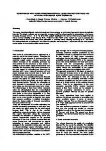
14 initially increases, then reaches a plateau and decreases; and the share of employment in services increases exponentially. In order to determine the best specification in the case of the KILM data set, several semi-parametric regressions between the share of employment in each economic sector and the per capita income were run. The results of this exercise are depicted in Figure 5.1.
Figure 5.1: Employment shares and per capita income by economic sector
Component+residual for INDUS
Fractional Polynomial (0 0)
Fractional Polynomial (3 3)
.942391 Component+residual for AGRIC
-.
025791 1.82689
.
lpcgdp
2.37374
642
-.05684 1.82689
lpcgdp
2.37374
Fractional Polynomial (-2 3) .
824506 Component+residual for SERV
.036 1.82689
lpcgdp
2.37374
The top left panel in Figure 5.1 shows the relationship between income and the employment share in agriculture; the top right for industry; the bottom left panel for the service sector. Overall, it is possible to say that these relationships reproduce the pattern found by Fuchs (1980) more than 20 years ago. These findings confirm that per capita GDP is a key predictor of economic structure. In what follows, the methodology applied above is adapted in order to deal with employment distribution by sector and the results of the predictions are described. Table 5.1 summarizes the response rates for employment by sector data across the different subregions. The global response rate is 44 per cent (slightly higher than for unemployment figures). Response rates of over 50 per cent apply to almost every subregion except sub-Saharan Africa, whose response rates are very low. This means we need to collapse this subregion with the Middle East and North Africa into one macro region. Several interpolation techniques were used to boost the response rates by filling the gaps between reported years for the respondent countries. Table 5.2 shows that the response rates increase very little.
15
Table 5.1: Response rates by subregion before interpolation 1991 1992 1993 1994 1995 1996 1997 1998 1999 2000 2001 2002 Total Major Europe
1.00
1.00
1.00
1.00
1.00
1.00
1.00
1.00
1.00
0.95
0.95
0.00
0.91
Major Non-Europe
1.00
1.00
1.00
1.00
1.00
1.00
1.00
1.00
1.00
1.00
1.00
0.00
0.92
Other Europe
0.50
0.50
0.50
0.50
0.50
0.00
0.00
0.00
0.50
1.00
1.00
0.00
0.42
Eastern Europe
0.33
0.33
0.42
0.58
0.58
0.67
0.67
0.67
0.67
0.67
0.67
0.00
0.52
Baltic States
0.67
0.67
0.67
0.67
0.67
0.67
1.00
1.00
1.00
1.00
1.00
0.00
0.75
CIS
0.58
0.58
0.67
0.67
0.67
0.58
0.67
0.67
0.75
0.42
0.33
0.00
0.55
Melanesia
0.67
0.67
0.67
0.33
0.33
0.33
0.33
0.33
0.00
0.00
0.00
0.00
0.31
Eastern Asia
0.86
0.86
0.86
0.86
0.86
0.86
0.86
0.71
0.71
0.71
0.43
0.00
0.71
South-Central Asia
0.50
0.50
0.50
0.50
0.63
0.38
0.25
0.25
0.13
0.38
0.00
0.00
0.33
South-Eastern Asia
0.55
0.73
0.82
0.64
0.64
0.55
0.64
0.55
0.45
0.36
0.18
0.00
0.51
Central America
0.74
0.74
0.74
0.79
0.79
0.79
0.79
0.84
0.68
0.53
0.53
0.16
0.68
South America
0.67
1.00
0.92
0.83
0.92
0.83
0.75
0.83
0.92
0.67
0.75
0.08
0.76
Eastern Africa
0.19
0.13
0.06
0.19
0.13
0.00
0.00
0.06
0.06
0.00
0.00
0.00
0.07
Middle Africa
0.00
0.00
0.00
0.00
0.00
0.00
0.00
0.00
0.00
0.00
0.00
0.00
0.00
Southern Africa
0.00
0.00
0.00
0.00
0.20
0.00
0.00
0.20
0.20
0.40
0.00
0.00
0.08
Western Africa
0.00
0.06
0.00
0.00
0.06
0.00
0.00
0.00
0.00
0.00
0.00
0.00
0.01
Middle East
0.13
0.13
0.13
0.13
0.20
0.20
0.13
0.13
0.20
0.20
0.13
0.00
0.14
North Africa
0.40
0.40
0.40
0.20
0.40
0.20
0.40
0.40
0.40
0.20
0.00
0.00
0.28
Total
0.48
0.51
0.51
0.51
0.54
0.48
0.49
0.50
0.49
0.43
0.37
0.02
0.44
Source: ILO, KILM, 3rd edition.
From Table 5.1 it can be concluded that there are missing values in every subregion (or region) and thus it is necessary to impute in every single geographic group. The estimation and imputation phase is similar to that applied for the unemployment rates. First, a missing values mechanism is estimated by running several logit regressions where the dependent variable is 1 if the country reports on distribution of employment by sector and 0 if the report is missing. The explanatory variables are those used in the case of unemployment rates. Several response probabilities are then predicted and country-level weights computed for the respondent countries. The results of this sequence of probit regressions are shown in Table 5.3. In eight out of the ten geographical groups, the assumption that missing values are missing completely at random is demonstrably rejected. Again, the per capita income and the size of the country are two important predictors of response probability. This implies that respondent countries are clearly different from non-respondent ones and that some gains can be obtained by weighting the sample of respondent countries.
16 Table 5.2: Response rates by subregion after interpolation 1991 1992 1993 1994 1995 1996 1997 1998 1999 2000 2001 2002 Total Major Europe Major Non-Europe Other Europe Eastern Europe Baltic States CIS Melanesia Eastern Asia South-Central Asia South-Eastern Asia Central America South America Eastern Africa Middle Africa Southern Africa Western Africa Middle East North Africa Total
1.00 1.00 0.50 0.33 0.67 0.58 0.67 0.86 0.50 0.55 0.74 0.67 0.19 0.00 0.00 0.00 0.13 0.40 0.48
1.00 1.00 0.50 0.33 0.67 0.58 0.67 0.86 0.50 0.73 0.74 1.00 0.19 0.00 0.00 0.06 0.13 0.40 0.52
1.00 1.00 0.50 0.42 0.67 0.67 0.67 0.86 0.50 0.82 0.79 0.92 0.19 0.00 0.00 0.00 0.13 0.40 0.53
1.00 1.00 0.50 0.58 0.67 0.67 0.33 0.86 0.50 0.73 0.79 0.92 0.25 0.00 0.00 0.00 0.13 0.40 0.53
1.00 1.00 0.50 0.58 0.67 0.67 0.33 0.86 0.63 0.73 0.79 0.92 0.13 0.00 0.20 0.06 0.20 0.40 0.54
1.00 1.00 0.50 0.67 0.67 0.67 0.33 0.86 0.50 0.64 0.79 0.92 0.06 0.00 0.20 0.00 0.27 0.40 0.53
1.00 1.00 0.50 0.67 1.00 0.67 0.33 0.86 0.50 0.64 0.79 0.92 0.06 0.00 0.20 0.00 0.20 0.40 0.53
1.00 1.00 0.50 0.67 1.00 0.67 0.33 0.71 0.50 0.55 0.84 0.92 0.06 0.00 0.20 0.00 0.20 0.40 0.53
1.00 1.00 0.50 0.67 1.00 0.75 0.00 0.71 0.38 0.45 0.79 0.92 0.06 0.00 0.40 0.00 0.27 0.40 0.52
0.95 1.00 1.00 0.67 1.00 0.42 0.00 0.71 0.38 0.36 0.63 0.83 0.00 0.00 0.40 0.00 0.20 0.20 0.46
0.95 1.00 1.00 0.67 1.00 0.33 0.00 0.43 0.00 0.18 0.58 0.75 0.00 0.00 0.00 0.00 0.13 0.00 0.38
0.00 0.00 0.00 0.00 0.00 0.00 0.00 0.00 0.00 0.00 0.16 0.08 0.00 0.00 0.00 0.00 0.00 0.00 0.02
0.91 0.92 0.54 0.52 0.75 0.56 0.31 0.71 0.41 0.53 0.70 0.81 0.10 0.00 0.13 0.01 0.17 0.32 0.46
Source: Author’s calculations.
Table 5.3 Determinants of response probability: Employment distribution by economic sector
PCGDP GROWTH SIZE
Developed
Developed
Europe
Non-Europe Europe
4.513 (3.55)** -0.096 (0.61) 1.282 (4.19)**
-20.073 (2.29)* 0.282 (0.84) 2.116 (2.04)*
-49.203 (3.66)** 231
182.056 (2.32)* 60
0.46 40.8**
0.2 6.4
HIPC Constant N Pseudo-R2 LR Chi2
Eastern CIS
0.206 (0.27) -0.094 (2.47)* 0.33 (1.40)
-0.714 (1.15) -0.003 (0.11) 1.158 (3.90)** 1.722 (2.57)* -5.451 -4.566 (0.74) (0.8) 143 132 0.15 26.4*
0.17 30.6**
Eastern
Central
South-East Central
South
Africa and
Asia
Asia
Asia
America
Middle East
3.036 (3.62)** 0.226 (1.75) 0.52 (2.22)* 8.269 (3.49)** -29.145 (3.36)** 77
2.16 2.254 2.443 -1.807 1.216 (3.09)** (4.54)** (5.30)** -1.35 (6.13)** -0.211 -0.115 -0.057 0.033 0.014 (1.12) (1.65) (0.94) -0.29 -0.68 0.294 0.916 0.837 1.386 0.705 (2.32)* (5.25)** (4.97)** (3.65)** (6.29)** -0.249 3.881 -4.71 0.642 (0.3) (3.64)** (3.36)** (1.43) -17.711 -24.726 -25.646 4.963 -17.867 (3.14)** (5.09)** (5.42)** -0.46 (7.86)** 80 154 228 132 715
0.59 48.3**
0.15 15.8
America
0.51 0.32 0.71 109.6** 90.24** 93.7**
Notes: Absolute value of the Z statistic is in parenthesis. (*) significant at 5%, (**) significant at 1%. N = No. of observations.
0.21 101.6**
17 After estimating the weights, the final step is to run a sequence of subregional weighted regressions. The prediction model is built on the basis of the empirical evidence summarized in Figure 5.1. That is, for each economic sector the following model for employment shares is estimated: ⎛ y YitkT = ln⎜⎜ itk ⎝ 1 − yitk
⎞ ⎟⎟ = α + xit' β + µ it ⎠
(17)
where yitk is the observed employment participation for economic sector k, country i and period t and xit is a set of covariates explaining this share. In this section this set of covariates includes both the level of the per capita income and its square value. One important difference here is that α is no longer country-specific. We proceeded in this way because, on the one hand, the inclusion of a fixed effect did not greatly affect the estimated correlations and, on the other, it did generate some implausible imputations in some subregions. One notable constraint to model (17) is that the add of the employment shares across all the economic sector should always add 1, that is:
∑y
itk
= 1 ∀i, t
(18)
k
As a consequence, model (17) was estimated as a system of equations for two sectors: agriculture and industry. The default sector is services, whose shares are computed as: yˆ itk = 1 − yˆ it ,agr − yˆ it ,ind ∀i, t
(19)
After estimation this model can be used for imputation and prediction. Although it is not strictly necessary to carry out imputations for non-respondent countries, doing so is useful to produce a “complete data set” that can be used in order to compute additional statistics of labour market conditions or to generate different regional and subregional aggregations. Tables 5.4 and 5.5 show the estimates and projections for the distribution of total employment by sector. One important point is that the model is able to impute ‘shares’ only; hence, to recover a total, some information about total employment will be needed. This figure is derived from the results on unemployment rates shown in previous sections. A negative side-effect of this approach is that the standard errors reported in Tables 5.4 and 5.5 will clearly be underestimated because they take as true a total employment value that was predicted with some error. In terms of the results, Table 5.5 suggests a reduction in employment, accounted for by the agricultural sector, from 42 per cent in 1996 to 20 per cent by 2015. This is a very significant drop and, as a consequence, agriculture is the only sector where a reduction in the absolute number of workers is expected. This fall for agriculture allows for a marginal increase in the participation of industry (from 22 per cent to 26 per cent) and, more remarkably, for a substantial increase in the service sector (from 37 per cent to 53 per cent). Therefore, although across the entire period it is expected that the total number of workers in industry will increase by about 300 million, the increased employment in services will be two times larger. Appendix tables A.16-A.21 present the same results by subregions. The pattern of change is always similar. Although a decrease in the participation of agriculture is confirmed for every subregion, important differences are observed across subregions. At one extreme are the countries of Eastern Asia where significant structural change is expected and where
18 the share of agriculture will fall from 57 per cent to 13 per cent by 2015, and at the other is the sub-Saharan African region, which is the most stable subregion and where a decrease from 48.5 per cent to just 47.2 per cent is expected. For the manufacturing sector, the patterns vary depending on the initial condition of the countries. We expect a fall in industrial employment in developed countries (Europe and Non-Europe), a rather stable situation in the middle-income countries of Central and South America and an increase in manufacturing employment in the rest of the world. This increase is expected to be relatively significant in South Central Asia (15 per cent to 28 per cent). As a consequence of these compensating trends, the world levels for manufacturing look fairly stable. Finally, all the countries will show growth in the participation of the service sector, particularly in East Asia where it is predicted to rise from 17 per cent in 1996 to 55 per cent by 2015), and also in South-Eastern Asia (37 per cent to 56 per cent). The remaining subregions will also show an increase but movements will be less dramatic. Table 5.4: Employment distribution by economic sector (‘000) Year Agriculture Standard deviation Industry Standard deviation Services Standard deviation
1996
1997
1998
1999
2000
2001
2002
2003
2004
2015
993981.5 1016692.2 1031457.9 1017261.3 1014201.0
948482.1
920249.8
911250.7
899601.8
651098.2
46914.3
47111.0
47317.5
47428.2
47619.6
47828.1
48151.5
48384.1
48650.6
30328.1
566703.4
564464.8
552916.7
562826.4
585472.0
621052.5
642225.4
661169.6
681875.9
876295.6
6845.7
6961.9
7130.4
7677.3
8134.3
8421.6
8874.9
9398.5
10100.2
18421.8
922831.9
949289.7
47411.2
47622.6
983401.2 1028806.1 1058839.8 1132319.4 1176714.3 1211930.9 1250697.2 1752359.0 47851.7
48045.6
48309.4
48563.8
48962.6
49288.4
49688.0
35484.6
Table 5.5: Employment distribution by economic sector (%) Year
1996
1997
1998
1999
2000
2001
2002
2003
2004
2015
Agriculture Standard deviation Industry Standard deviation Services Standard deviation
40.0 1.9 22.8 0.3 37.2 1.9
40.2 1.9 22.3 0.3 37.5 1.9
40.2 1.8 21.5 0.3 38.3 1.9
39.0 1.8 21.6 0.3 39.4 1.8
38.1 1.8 22.0 0.3 39.8 1.8
35.1 1.8 23.0 0.3 41.9 1.8
33.6 1.8 23.4 0.3 43.0 1.8
32.7 1.7 23.7 0.3 43.5 1.8
31.8 1.7 24.1 0.4 44.2 1.8
19.9 0.9 26.7 0.6 53.4 1.1
6. Conclusions
This report has proposed an integrated methodological approach aimed at generating imputations and projections from the KILM data set, which is a substantial undertaking designed by the ILO to collect and improve the coordination of data on various labour market indicators submitted by its member countries. The team responsible for KILM has concentrated first on widening geographical coverage and improving the timeliness of the information for the core indicators and, second, on expanding the set of indicators to further meet demand for realistic coverage of the world’s labour markets. The scope and complexity of the current data set affect the comparability of statistics among countries and regions.
19 Three shortcomings were detected: not all countries report information; many reporting countries report incomplete data; and, finally, not all the reported information is comparable across countries due to different methodological approaches. Improving the KILM data set will require more standardization of the different methodologies involved in data collection and processing than are currently being implemented by member countries. It will also necessitate achieving higher response rates. This entails a prolonged process of continuous investment, the results of which can only be looked for in the long term. Meanwhile, the methodological approach proposed in this investigation is designed to deal with the three shortcomings detected. The issue of incomplete information is overcome by the use of ad hoc country-level interpolation techniques. This also preserves much of the country-level heterogeneity. In addition, modelling the ‘missingness’ mechanism and weighting the sample of respondent countries deals with the issue of missing countries. The idea of introducing weights is to try to reduce the influence in the sample of those respondent countries that are vastly different. Finally, heterogeneity at country level was controlled for by adopting panel data techniques. The tests achieved from simulations of this approach are encouraging. A remarkable reduction of the bias in comparison with more standard alternatives is observed – with 50 per cent of bias reduction generated by the introduction of the weighting scheme used in the model, and the remaining 50 per cent resulting from working with fixed effects. Another significant result of the simulation is that this methodology preserves a large proportion of the original data variability. Of course, research into the consequences and properties of the suggested approach does not end with this investigation. Much still remains to be analysed, in particular how to achieve a more appropriate measurement of uncertainty. The present paper is only a minor step in this direction. A major advance would be to take into account (in the projections) the uncertainties that relate to the estimated fixed effects and, also, the proportion of observations that are imputed – as opposed to true – data. The method described in this report still treats the different dependent variables (such as unemployment sub-components) as single equations. Thus, all the information related to correlation among them is omitted, leading to an additional loss of information. More structural approaches will be necessary to deal with such issues. These alternative approaches would also require more highly sophisticated estimation techniques (such as maximum likelihood for incomplete data), and are beyond the scope of the present research. However, they must form part of the future research agenda.
20
Bibliograph FUCHS, V. 1980. "Economic growth and the rise of service employment," NBER Working Paper. HOROWITZ, J.; MANSKI, C.1998. "Censoring of outcomes and regressors due to survey nonresponse: Identification and estimation using weights and imputations," Journal of Econometrics, Vol. 84, No. 1, pp. 37-58. KILM. 2003. Key Indicators of the Labour Market, 3rd edition. Geneva, ILO. LITTLE, R., RUBIN, D. 1987: Statistical Analysis with Missing Data. New York, Wiley. SCHAFER, J.L. 1997. Analysis of Incomplete Multivariate Data. London, Chapman and Hall. SCHAIBLE, W. 2000: "Methods for producing world and regional estimates for selected key indicators of the labour market," Employment Sector Paper. Geneva, ILO. Available online at http://www.ilo.org/public/english/employment/strat/publ/ep00-6.htm SCHAIBLE, W.; MAHADEVAN-VIJAYA, R. 2002. "World and regional estimates for selected key indicators of the labour market". Employment Paper No. 2002/36. Available online at http://www.ilo.org/public/english/employment/strat/download/ep36.pdf
21
Appendix Table A.1: Total Male and Female Unemployment (‘000) MFU
1995
1996
1997
1998
1999
2000
2001
2002
2003
2004
2015
Europe
20258 0
20339 0
20181 0
19158 0
18278 0
16448 0
15354 0
16504 0
16542 313
16442 312
16428 314
Major Non-Europe
12052 0
12182 0
11577 0
11420 0
11286 0
10941 0
12324 0
14287 0
14496 328
14009 313
14782 338
6957
6703
6179
6153
6902
7615
7958
8366
8262
8363
7764
17
218
70
26
13
7
6
6
172
182
174
9183 24
9972 11
10957 15
12350 13
13581 18
10640 20
9768 23
9342 15
9142 1174
9136 1167
8190 1085
Eastern Asia
21134 1002
22475 935
23754 875
26403 805
27442 769
25570 833
27071 796
26151 853
27537 832
27893 843
27164 974
South Central Asia
25127 916
25438 892
23421 380
24275 427
26401 659
26027 394
25012 520
26233 419
27249 416
28898 497
33693 500
South-Eastern Asia
9307 195
9264 26
9301 23
11426 20
12301 24
12425 29
14335 24
16866 42
17178 260
17410 261
19933 276
Central America
4462 7
4042 4
3782 4
3608 3
3142 3
3123 5
3384 7
3465 23
3469 68
3424 67
3967 81
South America
9409 1
12318 1
12653 1
14544 1
17184 1
17107 1
15954 1
16528 160
16005 244
14658 220
17262 254
Sub-Saharan Africa
22706 206
23358 235
24777 220
25482 216
26047 181
27482 250
27991 212
29019 296
29663 328
29364 235
37816 282
Middle East
12807 64
12219 28
12899 67
13772 68
13740 82
14447 36
14474 34
14798 64
15284 119
15707 122
19097 144
Eastern Europe + Baltic
CIS
Total
153402 158310 159479 168592 176304 171825 173624 181558 184828 185304 206097 1388 1332 984 939 1033 956 975 1012 1653 1655 1693
Note: The standard deviation is given below unemployment estimates
.
22 Table A.2: Total Youth Male Unemployment (‘000) YMU
1995
1996
1997
1998
1999
2000
2001
2002
2003
2004
2015
Europe
3129 0
3024 0
2870 0
2732 0
2657 0
2328 0
2285 0
2510 0
2510 68
2477 67
2351 65
Major Non-Europe
2163 0
2203 0
2133 0
2095 0
2059 0
1966 0
2170 0
2382 0
2422 94
2352 92
2472 101
Eastern Europe + Baltic
1261
1140
1023
1019
1160
1221
1295
1341
1144
1135
821
5
34
14
6
3
1
2
2
54
55
38
CIS
1448 6
1524 5
1631 6
1791 7
1977 10
1542 10
1482 11
1367 8
1174 263
1185 263
821 162
Eastern Asia
6090 523
6283 469
6417 420
6815 371
6907 342
6379 365
6687 344
6455 370
6809 362
6954 370
6264 383
South Central Asia
10638 599
10645 580
9426 240
9971 270
10950 418
10625 246
10067 324
10637 263
11111 261
11901 313
13135 299
South-Eastern Asia
2990 136
3047 14
3062 12
3569 11
4192 13
4112 15
4717 12
5427 22
5489 180
5518 180
5733 181
Central America
1256 3
1129 2
1009 2
930 1
748 1
809 2
857 3
882 6
875 32
853 30
900 32
South America
2441 1
3176 0
3168 0
3646 1
4239 0
4117 1
3979 1
4096 76
3982 102
3599 94
3791 94
Sub-Sharan Africa
8608 113
8882 129
9438 129
9778 153
10084 134
10604 179
10727 154
11143 187
11444 219
11391 137
14845 178
Middle East
4240 38
4050 19
4254 41
4543 42
4409 51
4677 24
4650 20
4708 30
4845 67
4951 67
5191 61
44265 816
45103 758
44430 503
46889 485
49382 559
48380 476
48917 498
50948 499
51805 617
52315 621
56323 597
Total
Note: The standard deviation is given below unemployment estimates
23 Table A.3: Total Adult Male Unemployment (‘000) AMU
1995
1996
1997
1998
1999
2000
2001
2002
2003
2004
2015
Europe
7518 0
7739 0
7670 0
7179 0
6836 0
6117 0
5873 0
6560 0
6599 227
6581 226
6858 232
Major Non-Europe
4586 0
4614 0
4275 0
4287 0
4271 0
4156 0
4845 0
5765 0
5843 257
5633 243
5958 263
Eastern Europe + Baltic
2429
2384
2169
2219
2554
2794
2928
3101
3156
3221
3264
14
186
60
22
11
6
5
5
122
129
129
CIS
3534 17
3877 7
4254 10
4772 8
5268 11
3961 13
3660 15
3501 10
3495 821
3487 816
3480 792
Eastern Asia
7055 696
7747 666
8435 637
9832 598
10415 580
9722 631
10383 607
9985 648
10463 632
10549 639
11033 767
South Central Asia
4819 452
4931 445
4638 193
4816 218
5202 338
5179 206
5129 278
5371 222
5556 220
5840 260
7367 282
South-Eastern Asia
1885 37
1873 12
1924 11
2547 10
2584 12
2690 15
2973 12
3589 23
3694 78
3786 80
4897 104
Central America
1354 3
1179 2
998 2
977 1
895 1
874 2
951 3
982 5
985 42
973 41
1240 53
South America
2473 0
3250 0
3231 0
3663 1
4514 0
4555 1
4223 1
4256 57
4066 137
3610 118
4739 147
Sub-Saharan Africa
5557 122
5685 142
5970 127
5944 95
5961 82
6488 113
6524 86
6731 152
6805 156
6783 130
8869 154
Middle East
4290 44
4031 16
4253 44
4411 43
4532 51
4695 20
4700 18
4827 48
5003 83
5170 86
7269 115
45500 841
47309 835
47815 682
50647 645
53032 678
51229 674
52188 673
54670 706
55666 1146
55633 1147
64974 1227
Total
Note: The standard deviation is given below unemployment estimates
24 Table A.4: Total Youth Female Unemployment (‘000) YFU
1995
1996
1997
1998
1999
2000
2001
2002
2003
2004
2015
Europe
2730 0
2619 0
2575 0
2350 0
2234 0
1975 0
1772 0
1760 0
1742 44
1717 43
1559 39
Major Non Europe
1736 0
1740 0
1697 0
1635 0
1611 0
1527 0
1623 0
1802 0
1828 60
1802 60
1886 65
Eastern Europe + Baltic
999
935
858
816
908
947
1006
1064
1061
1057
755
3
22
8
3
2
1
1
1
34
36
24
CIS
1325 5
1396 4
1464 6
1579 4
1620 6
1482 7
1352 8
1325 5
1335 273
1340 274
875 166
Eastern Asia
4235 339
4302 300
4365 267
4552 233
4582 213
4255 227
4414 212
4285 229
4483 222
4563 226
4050 231
South Central Asia
5421 416
5362 399
5101 178
5115 193
5517 288
5762 175
5496 232
5636 182
5826 181
6090 210
6798 201
South-Eastern Asia
2657 129
2625 15
2534 13
3057 11
3310 12
3331 13
3908 11
4453 16
4500 155
4524 155
4686 155
953 4
860 2
850 2
820 2
712 2
681 3
779 4
796 15
799 26
790 26
824 28
South America
2206 0
2932 0
3021 0
3592 0
3995 0
4003 0
3823 0
3937 91
3817 107
3558 102
3748 100
Sub-Saharan Africa
5254 88
5407 94
5795 87
6069 107
6232 80
6541 117
6622 105
6894 134
7123 154
6940 98
8951 116
Middle East
2386 22
2343 10
2529 26
2787 27
2798 34
2924 14
2939 14
2976 17
3069 40
3141 41
3248 37
29902 560
30519 509
30788 334
32371 322
33519 369
33428 310
33734 332
34927 336
35583 474
35522 473
37379 421
Central America
Total
Note: The standard deviation is given below unemployment estimates
25 Table A.5: Total Adult Female Unemployment (‘000) AFY
1995
1996
1997
1998
1999
2000
2001
2002
2003
2004
2015
Europe
6882 0
6958 0
7066 0
6896 0
6551 0
6028 0
5424 0
5673 0
5691 200
5668 201
5660 198
Major Non-Europe
3567 0
3625 0
3472 0
3404 0
3345 0
3292 0
3685 0
4338 0
4403 171
4222 164
4466 176
Eastern Europe + Baltic
2267
2245
2129
2100
2281
2654
2730
2861
2902
2950
2923
8
105
33
12
6
3
3
3
103
110
107
CIS
2876 15
3175 5
3609 7
4209 6
4715 8
3655 9
3274 11
3149 7
3138 748
3123 742
3014 704
Eastern Asia
3753 362
4142 348
4537 334
5204 314
5539 306
5214 333
5587 321
5425 345
5782 335
5827 338
5818 401
South Central Asia
4250 319
4500 319
4255 131
4374 158
4731 252
4462 149
4320 184
4589 154
4756 155
5067 192
6393 201
South-Eastern Asia
1775 37
1720 11
1781 10
2252 9
2215 11
2293 14
2736 12
3398 22
3495 71
3583 73
4618 94
899 4
875 2
925 2
882 2
787 2
759 3
797 4
805 16
810 35
808 35
1004 44
South America
2289 0
2960 0
3233 0
3644 0
4436 0
4432 1
3929 0
4239 90
4140 136
3891 124
4985 155
Sub-Saharan Africa
3287 85
3384 97
3575 90
3690 52
3771 44
3850 64
4118 50
4251 107
4291 108
4250 98
5152 103
Middle East
1892 13
1796 7
1863 15
2031 14
2001 17
2150 9
2186 16
2286 26
2367 36
2446 38
3388 50
33735 492
35379 494
36446 372
38685 356
40371 399
38789 371
38785 374
41013 404
41775 902
41834 902
47420 909
Central America
Total
Note: The standard deviation is given below unemployment estimates
26 Table A.6: Male - Female Unemployment Rates (%) MFUR
1995 1996 1997 1998 1999 2000 2001 2002 2003 2004 2015
Europe
10.1 0
10.1 0
10 0
9.4 0
8.9 0
7.9 0
7.4 0
7.9 0
7.9 0.1
7.8 0.1
7.7 0.1
5.2 0
5.2 0
4.9 0
4.8 0
4.7 0
4.5 0
5.1 0
5.8 0
5.9 0.1
5.6 0.1
5.7 0.1
11.6
11.3
10.4
10.4
11.7
12.9
13.3
14
13.8
13.9
13.2
0
0.4
0.1
0
0
0
0
0
0.3
0.3
0.3
7 0
7.6 0
8.4 0
9.4 0
10.6 0
8.3 0
7.6 0
7.3 0
7.1 0.9
7 0.9
6.2 0.8
Eastern Asia
2.8 0.1
2.9 0.1
3 0.1
3.3 0.1
3.4 0.1
3.1 0.1
3.3 0.1
3.1 0.1
3.3 0.1
3.3 0.1
3 0.1
South Central Asia
5.4 0.2
5.3 0.2
4.8 0.1
4.8 0.1
5.1 0.1
4.9 0.1
4.6 0.1
4.8 0.1
4.8 0.1
5 0.1
4.6 0.1
South-Eastern Asia
4.2 0.1
4 0
4 0
4.8 0
5 0
4.9 0
5.5 0
6.3 0
6.3 0.1
6.3 0.1
5.9 0.1
Central America
7.3 0
6.5 0
5.8 0
5.4 0
4.6 0
4.5 0
4.8 0
4.9 0
4.8 0.1
4.6 0.1
4.3 0.1
South America
6.6 0
8.6 0
8.5 0
9.5 0
10.9 0
10.7 0
9.8 0
9.9 0.1
9.4 0.1
8.5 0.1
8.4 0.1
Sub-Saharan Africa
10.3 0.1
10.3 0.1
10.6 0.1
10.6 0.1
10.5 0.1
10.8 0.1
10.7 0.1
10.8 0.1
10.8 0.1
10.4 0.1
10.2 0.1
Middle East
13.3 0.1
12.3 0
12.5 0.1
12.9 0.1
12.3 0.1
12.6 0
12.3 0
12.2 0.1
12.2 0.1
12.2 0.1
11.3 0.1
Total
5.90 0.10
6.00 0.10
5.90 0.00
6.20 0.00
6.30 0.00
6.10 0.00
6.00 0.00
6.20 0.00
6.20 0.10
6.10 0.10
5.90 0.00
Major Non-Europe
Eastern Europe + Baltic
CIS
Note: The standard deviation is given below unemployment estimates
27 Table A.7: Youth Male Unemployment Rates (%) YMUR
1995 1996 1997 1998 1999 2000 2001 2002 2003 2004 2015
Europe
17.8 0
17.5 0
16.9 0
16 0
15.8 0
14 0
14 0
15.7 0
15.7 0.4
15.5 0.4
15.3 0.4
Major Non-Europe
11.4 0
11.7 0
11.3 0
11.1 0
10.9 0
10.4 0
11.6 0
12.7 0
12.8 0.5
12.4 0.5
12.5 0.5
Eastern Europe + Baltic
24.4
23.1
21.3
21.8
25.4
27.6
29.5
31.5
27.3
27.5
27.3
0.1
0.7
0.3
0.1
0.1
0
0
0
1.3
1.3
1.3
13.9 0.1
15.1 0.1
16 0.1
17.3 0.1
19.2 0.1
16.2 0.1
15.3 0.1
14.5 0.1
12.3 2.8
12.2 2.7
11 2.2
6.6 0.6
7 0.5
7.4 0.5
8.1 0.4
8.4 0.4
7.9 0.4
8.2 0.4
7.8 0.5
8.1 0.4
8.1 0.4
7.6 0.5
South Central Asia
14.4 0.8
14.2 0.8
12.4 0.3
12.9 0.3
13.9 0.5
13.2 0.3
12.3 0.4
12.7 0.3
13 0.3
13.6 0.4
12.9 0.3
South-Eastern Asia
9.4 0.4
9.3 0
9.4 0
11.4 0
12.4 0
12.1 0
13.6 0
15.5 0.1
15.5 0.5
15.4 0.5
15.4 0.5
Central America
10.9 0
9.7 0
8.7 0
7.9 0
6.5 0
7 0
7.5 0
7.8 0.1
7.6 0.3
7.4 0.3
7.2 0.3
South America
10.9 0
14.4 0
14 0
15.9 0
18.1 0
17.6 0
17.1 0
17.7 0.3
17.1 0.4
15.4 0.4
16.2 0.4
Sub-Saharan Africa
22.2 0.3
22.2 0.3
22.8 0.3
22.8 0.4
22.8 0.3
23.1 0.4
22.7 0.3
22.8 0.4
22.7 0.4
22 0.3
22.2 0.3
Middle East
24.8 0.2
23.1 0.1
23.4 0.2
24.1 0.2
22.2 0.3
23 0.1
22.6 0.1
22.7 0.1
22.7 0.3
22.7 0.3
22.4 0.3
Total
13.0 0.2
13.3 0.2
13.1 0.1
13.8 0.1
14.3 0.2
14.0 0.1
14.0 0.1
14.4 0.1
14.4 0.2
14.3 0.2
14.4 0.2
CIS
Eastern Asia
Note: The standard deviation is given below unemployment estimates
28 Table A.8: Adult Male Unemployment Rates (%) AMUR
1995 1996 1997 1998 1999 2000 2001 2002 2003 2004 2015
Europe
7.4 0
7.6 0
7.5 0
6.9 0
6.6 0
5.8 0
5.6 0
6.2 0
6.2 0.2
6.1 0.2
6.2 0.2
Major Non-Europe
4.2 0
4.1 0
3.8 0
3.8 0
3.7 0
3.6 0
4.2 0
4.9 0
4.9 0.2
4.7 0.2
4.8 0.2
Eastern Europe + Baltic
8.7
8.6
7.8
8
9.2
10.1
10.4
11
11.1
11.3
11.2
0
0.7
0.2
0.1
0
0
0
0
0.4
0.5
0.4
6 0
6.6 0
7.3 0
8.2 0
9.3 0
7 0
6.4 0
6.1 0
6.1 1.4
6 1.4
5.6 1.3
Eastern Asia
2.1 0.2
2.3 0.2
2.5 0.2
2.8 0.2
2.9 0.2
2.7 0.2
2.8 0.2
2.7 0.2
2.8 0.2
2.8 0.2
2.6 0.2
South Central Asia
1.9 0.2
1.9 0.2
1.7 0.1
1.8 0.1
1.9 0.1
1.8 0.1
1.8 0.1
1.8 0.1
1.8 0.1
1.9 0.1
1.8 0.1
South-Eastern Asia
1.9 0
1.9 0
1.9 0
2.4 0
2.4 0
2.4 0
2.6 0
3.1 0
3.1 0.1
3.1 0.1
3.1 0.1
Central America
4.7 0
3.9 0
3.2 0
3.1 0
2.8 0
2.6 0
2.8 0
2.8 0
2.7 0.1
2.6 0.1
2.6 0.1
South America
3.8 0
4.9 0
4.8 0
5.3 0
6.4 0
6.3 0
5.7 0
5.7 0.1
5.3 0.2
4.6 0.1
4.8 0.1
Sub-Saharan Africa
6.4 0.1
6.4 0.2
6.5 0.1
6.4 0.1
6.2 0.1
6.6 0.1
6.5 0.1
6.5 0.1
6.5 0.1
6.3 0.1
6.1 0.1
Middle East
7.6 0.1
6.9 0
7.1 0.1
7.2 0.1
7.1 0.1
7.2 0
7 0
7 0.1
7 0.1
7 0.1
7.1 0.1
Total
3.7 0.1
3.8 0.1
3.8 0.1
3.9 0.1
4.0 0.1
3.8 0.1
3.8 0.0
4.0 0.1
4.0 0.1
3.9 0.1
3.8 0.1
CIS
Note: The standard deviation is given below unemployment estimates
29 Table A.9: Youth Female Unemployment Rates (%) YFUR
1995 1996 1997 1998 1999 2000 2001 2002 2003 2004 2015
Europe
20.5 0
20.3 0
20.6 0
18.8 0
17.8 0
16 0
14.8 0
15.2 0
15 0.4
14.8 0.4
14.2 0.4
Major Non-Europe
10.4 0
10.5 0
10.2 0
9.7 0
9.6 0
9 0
9.7 0
10.7 0
10.8 0.4
10.5 0.3
10.7 0.4
Eastern Europe + Baltic
25.7
25.4
23.7
23
25.9
27.6
29.6
32
32.4
32.9
32.5
0.1
0.6
0.2
0.1
0
0
0
0
1.1
1.1
1
14.3 0
15.4 0
16.3 0.1
17.7 0
19.6 0.1
17.5 0.1
15.9 0.1
15.3 0.1
15.2 3.1
15.1 3.1
13.2 2.5
4.8 0.4
5 0.4
5.3 0.3
5.7 0.3
5.9 0.3
5.6 0.3
5.8 0.3
5.6 0.3
5.8 0.3
5.8 0.3
5.5 0.3
South Central Asia
15.7 1.2
15.5 1.2
14.6 0.5
14.5 0.5
15.6 0.8
16 0.5
15.4 0.7
15.7 0.5
15.9 0.5
16.3 0.6
15.9 0.5
South-Eastern Asia
10.9 0.5
10.8 0.1
10.6 0.1
12.8 0
13.8 0
13.5 0.1
15.6 0
17.6 0.1
17.6 0.6
17.6 0.6
17.7 0.6
Central America
16.1 0.1
14.5 0
13.9 0
13 0
11.4 0
10.9 0
12.6 0.1
12.9 0.2
12.8 0.4
12.6 0.4
12.4 0.4
South America
15.5 0
20.4 0
20.4 0
23.5 0
25.1 0
25 0
24 0
24.8 0.6
23.9 0.7
22.1 0.6
23 0.6
Sub-Saharan Africa
17.3 0.3
17.2 0.3
17.8 0.3
18 0.3
17.9 0.2
18.1 0.3
17.7 0.3
17.9 0.3
18 0.4
17 0.2
17.1 0.2
Middle East
34.5 0.3
32 0.1
32.7 0.3
34 0.3
31.4 0.4
32.9 0.2
32.4 0.2
32.5 0.2
32.6 0.4
32.6 0.4
32 0.4
Total
12.1 0.2
12.4 0.2
12.6 0.1
13.3 0.1
13.8 0.2
13.6 0.1
13.7 0.1
14.1 0.1
14.1 0.2
13.9 0.2
14.0 0.2
CIS
Eastern Asia
Note: The standard deviation is given below unemployment/employment estimates
30 Table A.10: Adult Female Unemployment Rates (%) AFUR
1995 1996 1997 1998 1999 2000 2001 2002 2003 2004 2015
Europe
10 0
10 0
10.1 0
9.7 0
9 0
8.2 0
7.3 0
7.6 0
7.6 0.3
7.5 0.3
7.5 0.3
Major Non-Europe
4.2 0
4.2 0
4 0
3.8 0
3.7 0
3.6 0
4 0
4.7 0
4.7 0.2
4.5 0.2
4.5 0.2
Eastern Europe + Baltic
9.7
9.7
9.2
9.1
9.8
11.3
11.5
11.9
12
12.2
12
0
0.5
0.1
0.1
0
0
0
0
0.4
0.5
0.4
CIS
5.4 0
6 0
6.8 0
7.8 0
9 0
6.9 0
6.1 0
5.9 0
5.8 1.4
5.8 1.4
5.4 1.3
Eastern Asia
1.5 0.1
1.6 0.1
1.7 0.1
1.9 0.1
1.9 0.1
1.8 0.1
1.9 0.1
1.8 0.1
1.9 0.1
1.9 0.1
1.7 0.1
South Central Asia
4.1 0.3
4.1 0.3
3.8 0.1
3.7 0.1
3.9 0.2
3.5 0.1
3.4 0.1
3.5 0.1
3.5 0.1
3.7 0.1
3.6 0.1
South-Eastern Asia
2.5 0.1
2.3 0
2.4 0
2.9 0
2.8 0
2.7 0
3.2 0
3.9 0
3.9 0.1
3.9 0.1
3.9 0.1
Central America
6.2 0
5.8 0
5.7 0
5.2 0
4.6 0
4.3 0
4.4 0
4.3 0.1
4.2 0.2
4.1 0.2
4 0.2
South America
5.6 0
7.2 0
7.4 0
8 0
9.2 0
9.1 0
7.8 0
8.2 0.2
7.8 0.3
7.1 0.2
7.4 0.2
Sub-Saharan Africa
5.1 0.1
5.1 0.1
5.2 0.1
5.2 0.1
5.2 0.1
5.2 0.1
5.4 0.1
5.4 0.1
5.4 0.1
5.2 0.1
4.8 0.1
11.9 0.1
10.7 0
10.6 0.1
11 0.1
10.3 0.1
10.7 0
10.3 0.1
10.4 0.1
10.4 0.2
10.4 0.2
10.3 0.2
4.2 0.1
4.3 0.1
4.3 0.0
4.5 0.0
4.6 0.0
4.3 0.0
4.2 0.0
4.4 0.0
4.4 0.1
4.3 0.1
4.2 0.1
Middle East
Total
Note: The standard deviation is given below unemployment estimates
31 Table A.11: Male - Female Employment-to-Population (%) MFUPOP
1995 1996 1997 1998 1999 2000 2001 2002 2003 2004 2015
Europe
50.4 0
50.1 0
50 0
50.6 0
51 0
51.5 0
51.6 0
51.2 0
51 0.1
51 0.1
48.9 0.1
Major Non-Europe
61.3 0
61.4 0
61.8 0
61.8 0
61.8 0
61.8 0
61.2 0
60.6 0
60.4 0.1
60.4 0.1
58.1 0.1
Eastern Europe + Baltic
52.5
51.8
51.8
51.3
50.4
49.4
49.3
48.8
48.8
48.7
48.3
0
0.2
0.1
0
0
0
0
0
0.2
0.2
0.2
57.1 0
56 0
55.3 0
54.4 0
52.2 0
53.1 0
53.4 0
53.4 0
53.4 0.5
53.4 0.5
54.2 0.5
78 0.1
77.9 0.1
77.8 0.1
77.4 0.1
77.3 0.1
77.2 0.1
77 0.1
76.9 0.1
76.6 0.1
76.4 0.1
74.3 0.1
South Central Asia
56.6 0.1
56.7 0.1
57.2 0
57.2 0.1
57.1 0.1
57.2 0
57.2 0.1
57 0
57 0
56.8 0.1
57.2 0
South-Eastern Asia
67.8 0.1
68.2 0
67.8 0
66.8 0
67.2 0
67.7 0
67.5 0
67 0
67.1 0.1
67.2 0.1
67.8 0.1
Central America
55.9 0
56.5 0
57.7 0
58.1 0
58.1 0
58 0
57.5 0
57.3 0
57.4 0.1
57.5 0.1
57.7 0.1
South America
61.5 0
59.6 0
60.4 0
60 0
59.9 0
59.5 0
60.2 0
59.8 0.1
60.2 0.1
60.8 0.1
60.5 0.1
Sub-Saharan Africa
66 0.1
66.1 0.1
65.9 0.1
66 0.1
66.1 0.1
66.1 0.1
66.1 0.1
66 0.1
66.1 0.1
66.3 0.1
67 0.1
Middle East
45 0
45.5 0
45.6 0
45.6 0
46.4 0
46 0
46 0
45.9 0
45.9 0.1
46 0
47.4 0
63.0 0.0
62.8 0.0
62.9 0.0
62.7 0.0
62.6 0.0
62.7 0.0
62.6 0.0
62.4 0.0
62.3 0.0
62.3 0.0
61.7 0.0
CIS
Eastern Asia
Total
Note: The standard deviation is given below employment estimates
32 Table A.12: Youth Male Employment-to-Population (%) YMUPOP
1995 1996 1997 1998 1999 2000 2001 2002 2003 2004 2015
Europe
44.1 0
44 0
44 0
45.1 0
44.8 0
45.5 0
44.6 0
43.2 0
43.1 0.2
43.2 0.2
43.3 0.2
Major Non-Europe
52.8 0
52.3 0
52.4 0
52.4 0
52.4 0
53 0
51.3 0
50.4 0
50.5 0.3
50.9 0.3
51.6 0.3
Eastern Europe + Baltic
37.9
36.6
36.3
35
32.7
30.8
29.9
28.5
30.1
29.9
29.7
0
0.3
0.1
0.1
0
0
0
0
0.5
0.5
0.5
41 0
38.6 0
38.2 0
37.7 0
36.2 0
34.3 0
34.6 0
33.4 0
34.3 1.1
34.5 1.1
37.4 0.9
Eastern Asia
71.7 0.4
71.1 0.4
70.4 0.4
69.2 0.3
68.4 0.3
68.3 0.3
67.5 0.3
67.4 0.3
67 0.3
67 0.3
69 0.3
South Central Asia
52.2 0.5
52.1 0.5
53 0.2
52.4 0.2
51.7 0.3
52.3 0.2
52.6 0.2
52.3 0.2
52.2 0.2
51.9 0.2
52.8 0.2
South-Eastern Asia
58.2 0.3
59 0
58.1 0
53.9 0
56.7 0
56.4 0
56.1 0
54.9 0
54.9 0.3
55 0.3
55.2 0.3
Central America
62.4 0
62.8 0
63.3 0
63.8 0
63.6 0
62.4 0
60.9 0
59.8 0
59.9 0.2
60.1 0.2
60.7 0.2
South America
63.8 0
59.6 0
60.1 0
58.4 0
57.1 0
56.6 0
56 0
54.8 0.2
55.2 0.3
56.4 0.3
54.9 0.3
Sub-Saharan Africa
56.1 0.2
56.2 0.2
55.8 0.2
55.9 0.3
56 0.2
56.2 0.3
56.4 0.2
56.3 0.3
56.4 0.3
57 0.2
57.4 0.2
Middle East
41.1 0.1
41.6 0.1
41.5 0.1
41.3 0.1
43 0.1
42.2 0.1
41.6 0.1
41 0.1
41.1 0.2
41.2 0.2
42.1 0.1
Total
56.8 0.2
56.2 0.1
56.0 0.1
55.1 0.1
54.9 0.1
54.7 0.1
54.3 0.1
53.8 0.1
53.8 0.1
54.0 0.1
55.0 0.1
CIS
Note: The standard deviation is given below employment estimates
33 Table A.13: Adult Male Employment-to-Population (%) AMUPOP
1995 1996 1997 1998 1999 2000 2001 2002 2003 2004 2015
Europe
66.5 0
65.9 0
65.8 0
66.2 0
66.1 0
66.5 0
66.4 0
65.8 0
65.7 0.1
65.5 0.1
62.7 0.1
75 0
75 0
75.2 0
75 0
74.8 0
74.6 0
73.8 0
72.9 0
72.7 0.2
72.7 0.2
69.1 0.2
66.1
65.6
65.6
65
63.9
62.8
62.8
62.2
62
61.8
59.7
0
0.5
0.2
0.1
0
0
0
0
0.3
0.3
0.3
CIS
71.8 0
70.7 0
69.4 0
68 0
65.6 0
66.7 0
67.2 0
67.3 0
67.3 1
67.3 1
66.4 0.9
Eastern Asia
87.7 0.2
87.4 0.2
87.1 0.2
86.7 0.2
86.4 0.1
86.5 0.2
86.2 0.1
86.2 0.2
85.9 0.1
85.8 0.1
83.3 0.2
South Central Asia
88.6 0.2
88.6 0.2
88.7 0.1
88.6 0.1
88.4 0.1
88.4 0.1
88.4 0.1
88.3 0.1
88.3 0.1
88.2 0.1
87.7 0.1
South-Eastern Asia
89.3 0
89.2 0
89 0
88.4 0
88.2 0
88.2 0
88 0
87.5 0
87.5 0.1
87.4 0.1
86.6 0.1
Central America
84.1 0
84.6 0
85.7 0
85.7 0
85.6 0
85.4 0
85 0
84.7 0
84.8 0.1
84.9 0.1
84.2 0.1
South America
83.8 0
82.1 0
82.5 0
82 0
81.1 0
80.8 0
81.3 0
81.1 0.1
81.4 0.2
81.9 0.1
80.5 0.1
Sub-Saharan Africa
87.5 0.1
87.4 0.1
87.1 0.1
87.2 0.1
87.2 0.1
86.8 0.1
86.8 0.1
86.7 0.1
86.7 0.1
86.9 0.1
87 0.1
Middle East
82.1 0.1
82.4 0
82.4 0.1
82.4 0.1
82.6 0.1
82.3 0
82.3 0
82 0.1
82 0.1
82 0.1
81.6 0.1
Total
82.6 0.1
82.4 0.1
82.3 0.0
82.1 0.0
81.8 0.0
81.9 0.0
81.8 0.0
81.6 0.0
81.5 0.1
81.5 0.1
80.5 0.1
Major Non-Europe
Eastern Europe + Baltic
Note: The standard deviation is given below employment estimates
34 Table A.14: Youth Female Employment-to-Population (%) YFUPOP
1995 1996 1997 1998 1999 2000 2001 2002 2003 2004 2015
Europe
33.7 0
33 0
32.2 0
33.2 0
33.9 0
34.2 0
33.7 0
32.8 0
32.8 0.1
32.9 0.1
32.8 0.1
Major Non-Europe
48.8 0
48.8 0
49.2 0
49.9 0
49.7 0
50.2 0
49.4 0
48.7 0
48.8 0.2
49.1 0.2
49.5 0.2
Eastern Europe + Baltic
29.2
27.6
27.7
27.4
26
24.9
24.2
23.1
22.9
22.6
22.4
0
0.2
0.1
0
0
0
0
0
0.4
0.4
0.3
37.3 0
35.6 0
34.5 0
33.2 0
29.6 0
30.7 0
30.9 0
31 0
31.1 1.1
31.2 1.1
33.3 1
74 0.3
73.4 0.3
72.7 0.2
71.6 0.2
70.8 0.2
70.4 0.2
69.6 0.2
69.4 0.2
69.1 0.2
69.1 0.2
70.6 0.2
South Central Asia
26.1 0.4
25.7 0.4
25.6 0.2
25.4 0.2
24.6 0.2
24.4 0.1
23.8 0.2
23.3 0.1
23.2 0.1
23.1 0.2
22.9 0.1
South-Eastern Asia
44.8 0.3
44.1 0
42.7 0
41.2 0
40.4 0
41.1 0
40.4 0
39.4 0
39.5 0.3
39.5 0.3
39.4 0.3
Central America
30.1 0
30.3 0
31.3 0
32.3 0
32.7 0
32.7 0
31.5 0
31 0.1
31 0.2
31.2 0.1
31.5 0.2
South America
39.1 0
36.4 0
37 0
36 0
36.2 0
36.1 0
36 0
35.2 0.3
35.7 0.3
36.6 0.3
36.4 0.3
Sub-Saharan Africa
46.3 0.2
46.6 0.2
46.5 0.2
46.6 0.2
46.8 0.1
47.1 0.2
47.4 0.2
47.3 0.2
47.3 0.2
47.9 0.1
48.3 0.1
15 0.1
16 0
16.1 0.1
16.2 0.1
17.7 0.1
16.7 0
16.7 0
16.5 0
16.5 0.1
16.5 0.1
16.8 0.1
43.7 0.1
42.9 0.1
42.2 0.1
41.5 0.1
40.9 0.1
40.7 0.1
40.1 0.1
39.7 0.1
39.7 0.1
39.8 0.1
39.5 0.1
CIS
Eastern Asia
Middle East
Total
Note: The standard deviation is given below employment estimates
35 Table A.15: Adult Female Employment-to-Population (%) AFUPOP
1995 1996 1997 1998 1999 2000 2001 2002 2003 2004 2015
Europe
40.2 0.1
40.2 0.1
40.1 0.1
40.8 0.1
41.5 0.1
42 0.1
42.5 0.1
42.4 0.1
42.3 0.1
42.1 0.1
39.6 0.1
53 0.1
53.2 0.1
53.8 0.1
53.8 0.1
53.9 0.1
53.9 0.1
53.7 0.1
53.3 0.1
53.1 0.1
53.1 0.1
50.4 0.1
49.1
48.7
48.6
48.3
48
47.2
47.2
47
46.8
46.5
44.5
0.3
0.4
0.3
0.2
0.2
0.2
0.2
0.2
0.2
0.2
0.2
CIS
53.2 0.4
52.7 0.7
52.5 0.7
52.2 0.7
50.2 0.8
51.8 0.9
52 0.8
52.3 0.8
52.2 0.8
52.1 0.8
50.2 0.7
Eastern Asia
71.5 0.1
71.7 0.1
72 0.1
71.9 0.1
72.1 0.1
71.9 0.1
72 0.1
71.9 0.1
71.6 0.1
71.3 0.1
67.2 0.1
South Central Asia
37.8 0.1
38.3 0.1
39 0
39.6 0.1
40 0.1
40.2 0
40.1 0.1
40 0
39.9 0
39.9 0.1
39.4 0
South-Eastern Asia
61.3 0
62.3 0.1
62.3 0.1
62.1 0.1
62.3 0.1
63.4 0.1
63.3 0.1
62.9 0.1
62.9 0.1
62.9 0.1
62.2 0.1
Central America
38.6 0.1
39.4 0.1
41 0.1
41.1 0.1
41.1 0.1
41.4 0.1
41.3 0.1
41.3 0.1
41.3 0.1
41.3 0.1
40.4 0.1
South America
48.4 0.1
47.4 0.1
48.8 0.1
49.1 0.1
50 0.1
49.4 0.1
50.9 0.1
50.7 0.1
50.9 0.1
51.3 0.1
50.3 0.1
Sub-Saharan Africa
61.7 0.1
62.1 0.1
62.2 0.1
62.5 0.1
62.6 0.1
62.7 0.1
62.7 0.1
62.7 0.1
62.7 0.1
62.8 0.1
63.3 0.1
Middle East
23.1 0.1
23.8 0.1
24.2 0.1
24.5 0.1
25.3 0.1
25.2 0
25.6 0
25.9 0
25.9 0
25.9 0
25.6 0
Total
52.6 0
52.9 0.1
53.3 0.1
53.4 0.1
53.6 0.1
53.8 0.1
53.9 0.1
53.8 0.1
53.7 0.1
53.5 0.1
51.4 0
Major Non-Europe
Eastern Europe + Baltic
Note: The standard deviation is given below employment estimates
36 Table A.16: Total Employment by Economic Sectors: Agriculture (‘000) Region Europe
Major Non-Europe
Eastern Europe + Baltic
1996
1997
1998
1999
2000
2001
2002
2003
2004
2015
16532.6 15839.7 16075.6 15997.2 14458.5 13672.6 15143.2 14974.4 14645.8 10541.5 773.6 735.1 782.2 814.2 772.2 833.2 778.7 771.4 763.7 516 8435.2 8312.2 8221.8 8065.9 180.8 191 199.7 228.9 11464.4 11411.8 11149.9 159.7
171.3
178.7
7987 272.7
7631 6998.2 6893.9 6686.8 4789.4 261.6 275.5 290.9 327.6 912.6
10830 10719.8
10689 7335.2
7029 6662.3 5514.7
175.9
155.1
145.1
165.7
147.8
28363 24099.1 28146.1 27702.5 29065.6 590.8 585.1 648 712.7 779
144.9
387.1
CIS
32886.8 28688.7 604.6 598.2
28740 28457.5 29908.1 862.4 952.4 1263.6
Eastern Asia
429231 433246. 450653. 456744. 462277. 387689. 377874. 368714. 358524. 113949. 5 2 3 8 2 6 2 5 7 46169 46326.3 46433.9 46447.7 46579.4 46733 47004.3 47171.9 47373 27195.6
South Central Asia 242593. 251332. 255309. 247944. 248535. 254265. 253222. 251557. 247573. 218973. 9 6 9 6 9 8 5 6 8 5 5954.1 6177.9 6468.1 7032.6 7372.3 7672.5 7989.4 8330.5 8677.7 11058.6 South-Eastern Asia
97891 108626. 103508. 91142.8 81971.6 70260.1 65786.7 66147.7 66216 56012.6 3 6 4455.9 4499.6 5017.5 5102.7 5128.2 5121.4 5099.6 5112.5 5095.1 4625.7
Central America
14378.3 377.7
15613 14759.9 14869.2 14835.4 14453.1 10780.9 10458.7 10614.3 11565.6 393.4 402.8 406.2 403.2 414.4 426.9 439.1 446.9 509.3
South America
20421.2 20805.4 20472 21767.8 10601.1 23846.2 12710.3 12270.3 12511.3 12185.2 961.6 983.9 1004.4 1024.5 1014.2 1050.9 1069.7 1083.9 1090.7 1017.1
Sub-Saharan Africa
98780 101769. 101374. 103178 109564. 112422. 114903. 117575. 120356. 157689. 6 9 8 7 5 2 3 3 3326.3 3439.7 3548.6 3624.6 3732.5 3840 3938.6 4031.8 4140 5542.3
Middle East
21367.1 21046.4 21569.1 22622.4 25102.9 25850 26429.2 26889.8 27353.1 29968.7 960.2 990.9 1014.9 1052 1049 1065.6 1086.1 1107.8 1129.3 1282.6
Note: The standard deviation is given below employment estimates
37
Table A.17: Total Employment by Economic Sectors: Industry (‘000) Region Europe
1996
1997
1998
52683.8 52560.2 53426.1 247.7
242.5
251.8
1999
2000
2001
53250 54070. 53881.3 8 257.4 257.1 263.6
2002
2003
2004
2015
53441 53649.8 53844.8 53218.6 256.7
257.9
260.3
293.9
Major Non-Europe 58478.3 59391.4 58853.7 58269.6 58437. 57031.1 54949.3 54964.6 54577.5 41121.7 7 1271.1 1364.6 1423.5 1758.5 2258.7 2134.9 2295.2 2465.3 2878.5 7990.5 Eastern Europe + Baltic
17568.2 17502.3 17348.2 16732.6 16200 113
117.3
121
124.5
126
16285 18116.1 18375.8 18610.4 20427.1 124.8
124.6
129.2
137.4
343.7
CIS
39101.5 34937.3 33678.5
Eastern Asia
196576. 195001. 180103. 178791. 18191 213300. 220420. 225529. 230977. 286515. 1 5 9 8 4 4 8 5 7 2 5371.3 5393.6 5414.3 5434.4 5478.6 5531.8 5616.4 5700.5 5808.5 8239.8
South Central Asia
31035 37354. 38521.2 38109.2 39108.7 39960.8 41030.9 2 1342.6 1323.9 1257.5 1355.3 1595.5 1821.6 2046.5 2319.3 2607.1 3539.8
69832 71350.4 74776.2 84591.9 91679. 93537.8 99623.7 106734. 115267. 198881. 4 3 1 9 3546.6 3699.1 3989 4725.1 5116.6 5482.3 5937.7 6458.2 7094.8 13724.8
South-Eastern Asia 41305.5 39709.7 36574.7 41929.7 42620. 46912 49900.5 51704.1 53702.7 83214.1 7 1031.5 1033.2 970.1 1015.3 1067.2 1077.6 1110.2 1147.7 1188.3 1904.9 Central America
South America
13150.9 13576.1 15481.3 15283.4 16096. 15960.3 15060.8 15451.5 15824.5 7 198.1 212.8 221.4 230.5 244.3 242.4 243.3 249.5 258.5 29386.1 30521.5 30421.7 29552.1 33341. 30287.5 35465.7 36477.4 1 382.4 409.9 418.9 412.2 413 409.1 403.2 413.5
Sub-Saharan Africa 26143.7 691.4 Middle East
26685 28305.1 28152.7 29277. 30182.9 3 709.7 730.4 755.2 777.6 795.6
22477.4 23229.3 23947.3 25237.7 24480. 1 463.1 471.2 481 497.3 518
Note: The standard deviation is given below employment estimates
19129 358
37614 46637.3 423.9
677.9
31049 31985.7 33195.2 43751.1 816.3
839
864.5 1164.6
25153 26089.3 27188.3 28301.2 42368.6 535.2
553
577.6
603.3
970.1
38 Table A.18: Total Employment by Economic Sectors: Services (‘000) Region
1996
1997
1998
1999
2000
Europe
111918.7 113620.9 116134.3 812.3 774.1 821.7
Major NonEurope
153695.8 156728.8 159644.9 162603.4 165034.4 1283.9
1377.9
Eastern Europe + 23706.2 24095.8 195.6 207.6 Baltic CIS
1437.4
2001
2002
2003
2004
2015
118912 122711.9 125244.4 123851.8 124591.2 125562.3 132281.9 853.9 813.9 873.9 819.9 813.4 806.8 593.8
1773.3
2275.1
24349 24682.3 24578.4 215.8 215.5 208.2
166715 169094.1 170791.1
173604 200200.8
2150.8
2897.1
2311.7
2482.4
24694 25963.2 26272.4 199 193.3 194.3
8042.4
26455 25278.4 199.7 517.7
48883.8 56347.3 56707.2 59385.4 51802.4 52537.4 52308.5 52503.8 52615.7 1472.4 1452.8 1389.4 1476.2 1722.1 1956.1 2189.7 2474.4 2775.6
52425 3758.5
Eastern Asia
127360.5 133586 137344.7 141265.6 143299.7 195662.7 210134.8 223499.4 238283.5 492394.3 46480.4 46639.3 46748.5 46764.6 46900.5 47059.3 47338.6 47515.1 47727.8 28416.5
South Central Asia
140342.3 144374.8 148917.8 157096.2 162093.4 166006.6 171538.6 177894.5 184730.3 274556.5 6930.3
South-Eastern Asia
7599.2
8472.6
8973.9
82226.8 77148.9 87036.2 100612.7 116269.4 4573.7
Central America
7200.7
4616.6
5110.4
31004 31997.2 32722.8 426.5 447.3 459.6
5202.8
5238
9429.9
9954.3 10540.7 11208.9 17625.6
128303 133113.9 136482.6 140031.1 178735.8 5233.6
5219.1
5239.7
5231.8
5002.6
34303 34893.8 36274.8 42051.5 43612.2 44757.7 56941.7 467 471.4 480.1 491.4 505.1 516.3 622.5
South America
81457.4 84755.2 87235.1 89628.2 98984.6 93443.2 101489.5 104750.2 107995.5 129352.1 1034.8 1065.9 1088.3 1104.3 1095.1 1127.7 1143.2 1160.1 1170.2 1222.3
Sub-Saharan Africa
78722.8 80557.3 85428.2 90020.2 3397.4 3512.1 3623 3702.4
Middle East
43513.6 46077.5 1066 1097.2
47881 1123.1
88458 90963.6 93405.2 3812.6 3921.5 4022.3
96065 99408.9 4118.2 4229.3
132476 5663.3
50297 50713.8 52474.6 53763.2 55468.4 57253.1 77716.6 1163.7 1169.9 1192.5 1218.8 1249.4 1280.3 1608.2
Note: The standard deviation is given below employment estimates
39
Table A.19: Total Employment by Economic Sectors: Agriculture (%) Region
1996 1997 1998 1999 2000 2001 2002 2003 2004 2015
Europe
9.1 0.4
8.7 0.4
8.7 0.4
8.5 0.4
7.6 0.4
7.1 0.4
7.9 0.4
7.8 0.4
7.5 0.4
5.4 0.3
Major Non-Europe
3.8 0.1
3.7 0.1
3.6 0.1
3.5 0.1
3.5 0.1
3.3 0.1
3.0 0.1
3.0 0.1
2.8 0.1
1.9 0.4
Eastern Europe + Baltic
21.7 0.3
21.5 0.3
21.1 0.3
20.7 0.3
20.8 0.3
20.7 0.3
14.3 0.3
13.6 0.3
12.9 0.3
10.8 0.8
CIS
27.2 0.5
23.9 0.5
23.9 0.5
21.0 0.5
24.0 0.6
23.3 0.6
24.3 0.7
23.9 0.7
23.5 0.8
24.2 1.0
Eastern Asia
57.0 6.1
56.9 6.1
58.7 6.0
58.8 6.0
58.7 5.9
48.7 5.9
46.7 5.8
45.1 5.8
43.3 5.7
12.8 3.0
South Central Asia
53.6 1.3
53.8 1.3
53.3 1.4
50.6 1.4
49.5 1.5
49.5 1.5
48.3 1.5
46.9 1.6
45.2 1.6
31.6 1.6
South-Eastern Asia
44.2 2.0
48.2 2.0
45.6 2.2
39.0 2.2
34.0 2.1
28.6 2.1
26.4 2.0
26.0 2.0
25.5 2.0
17.6 1.5
Central America
24.6 0.6
25.5 0.6
23.4 0.6
23.1 0.6
22.5 0.6
21.7 0.6
15.9 0.6
15.0 0.6
14.9 0.6
13.2 0.6
South America
15.6 0.7
15.3 0.7
14.8 0.7
15.4 0.7
7.4 0.7
16.2 0.7
8.5 0.7
8.0 0.7
7.9 0.7
6.5 0.5
Sub-Saharan Africa
48.5 1.6
48.7 1.6
47.1 1.6
46.6 1.6
48.2 1.6
48.1 1.6
48.0 1.6
47.9 1.6
47.6 1.6
47.2 1.7
Middle East
24.5 1.1
23.3 1.1
23.1 1.1
23.0 1.1
25.0 1.0
25.0 1.0
24.9 1.0
24.5 1.0
24.2 1.0
20.0 0.9
Note: The standard deviation is given below employment estimates
40
Table A.20: Total Employment by Economic Sectors: Industry (%) Region
1996 1997 1998 1999 2000 2001 2002 2003 2004 2015
Europe
29.1 0.1
28.9 0.1
28.8 0.1
28.3 0.1
28.3 0.1
27.9 0.1
27.8 0.1
27.8 0.1
27.7 0.1
27.1 0.1
Major Non-Europe
26.5 0.6
26.5 0.6
26 0.6
25.5 0.8
25.2 1
24.6 0.9
23.8 1
23.6 1.1
23.2 1.2
16.7 3.2
Eastern Europe + Baltic
33.3 0.2
33 0.2
32.8 0.2
32 0.2
31.5 0.2
31.5 0.2
35.2 0.2
35.6 0.3
36 0.3
39.9 0.7
CIS
32.3 1.1
29.1 1.1
28.4 1.1
27.1 1.2
31.8 1.4
32.4 1.5
31.9 1.7
32.5 1.9
33 2.2
33.3 2.9
Eastern Asia
26.1 0.7
25.6 0.7
23.4 0.7
23 0.7
23.1 0.7
26.8 0.7
27.3 0.7
27.6 0.7
27.9 0.7
32.1 0.9
South Central Asia
15.4 0.8
15.3 0.8
15.6 0.8
17.3 1
18.3 1
18.2 1.1
19 1.1
19.9 1.2
21.1 1.3
28.7 2
South-Eastern Asia
18.7 0.5
17.6 0.5
16.1 0.4
17.9 0.4
17.7 0.4
19.1 0.4
20.1 0.4
20.3 0.5
20.7 0.5
26.2 0.6
Central America
22.5 0.3
22.2 0.3
24.6 0.4
23.7 0.4
24.5 0.4
23.9 0.4
22.2 0.4
22.2 0.4
22.2 0.4
21.8 0.4
South America
22.4 0.3
22.4 0.3
22 0.3
21 0.3
23.3 0.3
20.5 0.3
23.7 0.3
23.8 0.3
23.8 0.3
24.8 0.4
Sub-Saharan Africa
12.8 0.3
12.8 0.3
13.2 0.3
12.7 0.3
12.9 0.3
12.9 0.3
13 0.3
13 0.3
13.1 0.3
13.1 0.3
Middle East
25.7 0.5
25.7 0.5
25.6 0.5
25.7 0.5
24.4 0.5
24.3 0.5
24.5 0.5
24.8 0.5
25.1 0.5
28.2 0.6
Note: The standard deviation is given below employment estimates
41 Table A.21: Total Employment by Economic Sectors: Services (% Region
1996 1997 1998 1999 2000 2001 2002 2003 2004 2015
Europe
61.8 0.4
62.4 0.4
62.6 0.4
63.2 0.5
64.2 0.4
65.0 0.5
64.4 0.4
64.5 0.4
64.7 0.4
67.5 0.3
Major Non-Europe
69.7 0.6
69.8 0.6
70.4 0.6
71.0 0.8
71.3 1.0
72.1 0.9
73.2 1.0
73.4 1.1
73.9 1.2
81.3 3.3
Eastern Europe + Baltic
45.0 0.4
45.5 0.4
46.1 0.4
47.2 0.4
47.7 0.4
47.8 0.4
50.5 0.4
50.8 0.4
51.1 0.4
49.4 1.0
CIS
40.4 1.2
47.0 1.2
47.8 1.2
51.9 1.3
44.2 1.5
44.2 1.6
43.8 1.8
43.6 2.1
43.5 2.3
42.5 3.0
Eastern Asia
16.9 6.2
17.5 6.1
17.9 6.1
18.2 6.0
18.2 6.0
24.6 5.9
26.0 5.9
27.3 5.8
28.8 5.8
55.1 3.2
South Central Asia
31.0 1.5
30.9 1.5
31.1 1.6
32.1 1.7
32.3 1.8
32.3 1.8
32.7 1.9
33.2 2.0
33.7 2.0
39.7 2.5
South-Eastern Asia
37.1 2.1
34.2 2.0
38.3 2.3
43.1 2.2
48.3 2.2
52.3 2.1
53.5 2.1
53.7 2.1
53.9 2.0
56.2 1.6
Central America
53.0 0.7
52.3 0.7
52.0 0.7
53.2 0.7
53.0 0.7
54.4 0.7
61.9 0.7
62.7 0.7
62.9 0.7
65.0 0.7
South America
62.1 0.8
62.3 0.8
63.2 0.8
63.6 0.8
69.3 0.8
63.3 0.8
67.8 0.8
68.2 0.8
68.3 0.7
68.7 0.6
Sub-Saharan Africa
38.7 1.7
38.5 1.7
39.7 1.7
40.7 1.7
38.9 1.7
38.9 1.7
39.0 1.7
39.1 1.7
39.3 1.7
39.7 1.7
Middle East
49.8 1.2
51.0 1.2
51.3 1.2
51.2 1.2
50.6 1.2
50.7 1.2
50.6 1.1
50.6 1.1
50.7 1.1
51.8 1.1
Note: The standard deviation is given below employment estimates
EMPLOYMENT STRATEGY PAPERS
2004/1
Macroeconomic reforms and a labour policy framework for India, by Jayati Ghosh
2004/2
Macroeconomic reforms, labour markets and labour policies: Chile, 1973-2000, by Guillermo Campero
2004/3
Employment and labour market effects of globalization: Selected issues for policy management, by Haroon Bhorat and Paul Lundall
2004/4
Successful employment and labour market policies in Europe and Asia and the Pacific, by Claire Harasty (ed.)
2004/5
Global poverty estimates and the millennium goals: Towards a unified framework, by Massoud Karshenas
2004/6
The labour market effects of US FDI in developing countries, by Robert E. Lipsey
2004/7
Industrial relations, social dialogue and employment in Argentina, Brazil and Mexico, by Adaberto Cardoso
2004/8
Global employment trends for women, 2004, by Sara Elder and Dorothea Schmidt
2004/9
Agricultural productivity growth, employment and poverty in developing countries, 1970-2000, by D.S. Prasada Rao, Timothy J. Coelli and Mohammad Alauddin
2004/10
Efectos de la apertura comercial en el empleo y el mercado laboral de México y sus diferencias con Argentina y Brasil (1990-2003), by Enrique Dussel Peters
2004/11
Capital inflows and investment in developing countries, by Ajit K. Ghose
2004/12
Reaching Millennium Goals: How well does agricultural productivity growth reduce poverty?, by Nomaan Majid
2004/13
Labour market policies and regulations in Argentina, Brazil and Mexico: Programmes and impacts, by Adriana Marshall
2004/14
Estimating growth requirements for reducing working poverty: Can the world halve working poverty by 2015?, by Steven Kapsos
2004/15
Insights into the tenure-productivity-employment relationship, by Peter Auer, Janine Berg and Ibrahima Coulibaly
2004/16
Imputation, estimation and prediction using the Key Indicators of the Labour Market (KILM) data set, by Gustavo Crespi Tarantino
These papers may be downloaded from our website at www.ilo.org/public/english/employment/strat/espapers.htm