Jan 31, 2009 - Mixture Models. Conference on Computer Vision and Pattern Recognition. 2008. Ryan Gomes (CalTech). Piero
A summary of
Incremental Learning of Nonparametric Bayesian Mixture Models Conference on Computer Vision and Pattern Recognition 2008
Ryan Gomes (CalTech) Piero Perona (CalTech) Max Welling (UCI)
Motivation • Unsupervised learning with very large datasets • Requirements • Model of evolving complexity • Limits on space and time
Overview Estimate Model Document 1 2
Document 1
1.5 1 0.5 0 !0.5 !1
Document 2
2 !1.5 1.5 !2 !2 1
Document 2 !1.5
!1
!0.5
0
0.5
1
1.5
2
!1.5
!1
!0.5
0
0.5
1
1.5
2
0.5 0 !0.5 !1 !1.5 !2 !2
Overview Estimate Model
Compression
Document 1 2
Document 1
Document 1
1.5 1 0.5 0 !0.5 !1
Document 2
2 !1.5 1.5 !2 !2 1
Document 2
Document 2 !1.5
!1
!0.5
0
0.5
1
1.5
2
!1.5
!1
!0.5
0
0.5
1
1.5
2
0.5 0 !0.5 !1 !1.5 !2 !2
Overview Estimate Model
Compression
Get more data, estimate model
Document 1
Document 1
Document 2
Document 2
Document 1 2
Document 1
1.5 1 0.5 0 !0.5 !1
Document 2
2 !1.5 1.5 !2 !2 1
Document 2 !1.5
!1
!0.5
0
0.5
1
1.5
2
0.5 0 !0.5 !1 Document 3
!2 !2
Document 3
2
!1.5
1.5
!1.5
!1
!0.5
0
0.5
1
1.5
2 1 0.5 0 !0.5 !1
Document 4
Document 4
2 !1.5 1.5
!2 !2 1
!1.5
!1
!0.5
0
0.5
1
1.5
2
0.5 0 !0.5 !1 !1.5 !2 !2
!1.5
!1
!0.5
0
0.5
1
1.5
2
Overview Estimate Model
Compression
Get more data, estimate model
Compression
Document 1
Document 1
Document 1
Document 2
Document 2
Document 2
Document 1 2
Document 1
1.5 1 0.5 0 !0.5 !1
Document 2
2 !1.5 1.5 !2 !2 1
Document 2 !1.5
!1
!0.5
0
0.5
1
1.5
2
0.5 0 !0.5 !1 Document 3
!2 !2
Document 3
2
!1.5
Document 3
1.5
!1.5
!1
!0.5
0
0.5
1
1.5
2 1 0.5 0 !0.5 !1
Document 4
Document 4
2 !1.5
Document 4
1.5
!2 !2 1
!1.5
!1
!0.5
0
0.5
1
1.5
2
0.5 0 !0.5 !1 !1.5 !2 !2
!1.5
!1
!0.5
0
0.5
1
1.5
2
Overview Model Building Phase Estimate Model
SMEM (Split & merge EM) algorithm
Document 1 2
Document 1
1.5
SMEM Algorithm for Mixture Models N.Ueda 1999
1 0.5 0 !0.5 !1
Document 2
2 !1.5 1.5 !2 !2 1
Document 2 !1.5
!1
!0.5
0
0.5
1
1.5
2
!1.5
!1
!0.5
0
0.5
1
1.5
2
0.5 0 !0.5 !1 !1.5 !2 !2
1. Rank splits and merges 2. Try 10 best splits 3. Try 10 best merges 4. Do best split or merge 5. Repeat 2-3-4 until free energy converges
Overview Compression Phase Estimate Model
Compression
Document 1 2
Document 1
Document 1
1.5 1 0.5 0 !0.5 !1
Document 2
2 !1.5 1.5 !2 !2 1
Document 2
Document 2 !1.5
!1
!0.5
0
0.5
1
1.5
2
!1.5
!1
!0.5
0
0.5
1
1.5
2
0.5 0 !0.5 !1 !1.5 !2 !2
1. Hard cluster data 2. Find the best cluster to split 3. Split cluster 4. Repeat 2-3 until memory constraint 5. Create clumps delete data points
Overview Model Building Phase Estimate Model
Compression
Get more data, estimate model
Document 1
Document 1
Document 2
Document 2
Document 1 2
Document 1
1.5 1 0.5 0 !0.5 !1
Document 2
2 !1.5 1.5 !2 !2 1
Document 2 !1.5
!1
!0.5
0
0.5
1
1.5
2
0.5 0 !0.5 !1 Document 3
!2 !2
Document 3
2
!1.5
1.5
!1.5
!1
!0.5
0
0.5
1
1.5
2 1 0.5 0 !0.5 !1
Document 4
Document 4
2 !1.5 1.5
!2 !2 1
!1.5
!1
!0.5
0
0.5
1
1.5
2
0.5 0 !0.5 !1 !1.5 !2 !2
!1.5
!1
!0.5
0
0.5
1
1.5
2
Overview Compression Phase Estimate Model
Compression
Get more data, estimate model
Compression
Document 1
Document 1
Document 1
Document 2
Document 2
Document 2
Document 1 2
Document 1
1.5 1 0.5 0 !0.5 !1
Document 2
2 !1.5 1.5 !2 !2 1
Document 2 !1.5
!1
!0.5
0
0.5
1
1.5
2
0.5 0 !0.5 !1 Document 3
!2 !2
Document 3
2
!1.5
Document 3
1.5
!1.5
!1
!0.5
0
0.5
1
1.5
2 1 0.5 0 !0.5 !1
Document 4
Document 4
2 !1.5
Document 4
1.5
!2 !2 1
!1.5
!1
!0.5
0
0.5
1
1.5
2
0.5 0 !0.5 !1 !1.5 !2 !2
!1.5
!1
!0.5
0
0.5
1
1.5
2
Technical details Dirichlet mixture model
•
•
Define variables
Model Building
•
•
•
Inheriting clump constraints
•
Constrained free energy
Compression Phase •
Top-down clustering
•
Memory cost computation
Topic Model !
"
joint probability
p(x, z, η, π, α) =
! ij
z
! k
#
x
xij : zij : ηk : πj : α: β : a, b :
observation model
mixture weight
p(xij |zij ; η)πj,zij p(η k |β)G(αk ; a, b)
prior on mixture components
gamma prior on Dirichlet hyper-param
word i in document j topic assignment variable for word i in document j parameter for topic k mixture of topics for document j (with Dirichlet prior) topic mixture prior parameter (with Gamma priors) topic prior hyperparameter Gamma prior hyperparameters
"
j
D(πj ; α)
Dirichlet topic mixture prior
estimate mod
Overview
Document 1 2 1.5
Document 1
Document 1
Document 1
1
Estimate Model
0.5
Get more data, estimate model
Compression
0 !0.5 !1
Document 1 2 1.5
0.5
Document 1 Document 2
Document 1 Document 2
1.5 !2 !2 1
1
!1.5
!1
!0.5
0
0.5
1
1.5
Document Docum 2
2
0.5
0
0
!0.5
!0.5
!1
!1
Document 2
2 !1.5 1.5 !2 !2 1
Document 2
2 !1.5
Document 1
Compr
Document 2 !1.5
!1
!0.5
0
0.5
1
!2 1.5 !2 2 !1.5
Document 3
Document 2
Document 2
!1.5
1.5
!1
!0.5
0
0.5
1
1.5
2 1
0.5
0.5
Model Building Phase 0
0
!0.5
!0.5
!1
!1
Document 3
Document 3
2
!1.5
!2 !2
Document Docum 3
2
1.5
1.5
!1.5
!1
!0.5
0
0.5
1
1.5
!2 !2 1
2 1 0.5
0.5
0
0
!1
!0.5
0
0.5
!1
!1
Document 4
Document 4
2 !1.5
!1.5
!1
!0.5
0
Docum
!1.5
1.5
0.5
1
1.5
!2 !2
0.5 0 !0.5 !1 !1.5 !2 !2
!1.5
!0.5
!0.5
!2 !2 1
Document 4
Document Docum 4
2 !1.5
!1.5
!1
!0.5
0
0.5
1
1.5
2
2
!1.5
!1
!0.5
0
0.5
1
Variational inference (general formulation)
observed variables
L(X) ≥ B(X)
marginal data likelihood
B(X) =
!
W
hidden variables
Lower bound (Free Energy)
joint probability
q(W ) log variational distribution (next page)
p(W,X) q(W )
mean-field variational approximation (generic truncated version)
q(v , η , z) = ∗
∗
!T
t=1 qγt (vt ) stick lengths
Beta distribution In this paper→ qγt (vt ) = Beta(γt,1 , γt,2 )
!T
t=1 qτt (ηt ) mixture components
!N
Inverse Normal Wishart distribution
n q (z ) n=1 φn responsibilities (topic assignments)
multinomial distribution
Recall that stick lengths are used to compute mixing weights
πi (ν ) = νi ∗
!i−1
j=1 (1
− νj )
derivation of lower bound (DP mixture model)
log p(x; α, λ)
=
log ×
! " z
#N
v
∗
"
∗ ∗ p(ν |α)p(η |λ) η Beta prior on Inverse Wishart prior ∗
mixture weights on mixture components
∗ ∗ ∗ p(x |η )p(z |ν )dν dη n z n n n=1 multinomial Gaussian observation mixture topic weight model
≥ Eq(ν ∗ ,η ∗ ,z) [log p(ν ∗ |α)p(η ∗ |λ) ×
#N
∗ p(x |η )p(z |ν )] n z n n n=1
Jensen’s inequality
Free Energy (unconstrained using all data points)
F
=
!T
"
t=1 Eqγt log
+ +
!T
"
qγt (νt ) p(νt |α)
t=1 Eqτt log
!N
"
qτt (ηt ) p(ηt |λ)
n=1 Eqφn log
* N: total number of data points * T: number of topics/latent states (T for “truncation”)
#
#
qφn (zn ) p(xn |ηzn )p(zn |ν ∗ )
#
“Clumps” if xij and xi! j! are in clump c: q(zij ) = q(zi! j ! ) = q(zc ) if xij and xi! j ! in clump c Document 1 2
Document 1
Document 1
1.5 1 0.5 0 !0.5 !1
Document 2
2 !1.5 1.5 !2 !2 1
Document 2
Document 2
!1.5
!1
!0.5
0
0.5
1
1.5
2
0.5 0 !0.5 !1
!
!1.5
Key assumption: !2 !2
!1.5
!1
p(xij |ηzij ) in exponential family with conjugate prior p(ηk |β)
!0.5
0
0.5
1
1.5
2
Constrained Free Energy “Lower bound on the lower bound” FC
= − −
!K
k=1
!K
+N T
k=1
!
s
Data multiplier
KL(qγk (νk )||p(νk |α)) KL(qτ (ηk )||p(ηk |λ)) ns log
!K
k=1
exp(Ssk )
s: clump index n_s: number of data points represented by clump s *Change in notation T → K (K: total number of mixture components now) * N and T have new meanings (N: number of expected data points in the future, T: number of data points now)
Update equations γk1
= α1 +
N T
γk2
= α2 +
N T
τk1
= λ1 +
N T
τk2
= λ2 +
N T
!
s
!
ns q(zs = k) !K
q(zs = j)
s
ns
s
ns q(zs = k)!F (x)"s
! !
s
j=k+1
ns q(zs = k)
q(zs = k) = !Kexp(Ssk ) j=1
exp(Ssj )
Ssk = Eq(V,φk ) log {p(zs = k|V )p(!F (x)"s |φk )}
generic procedure for computing variational parameter updates is given in [Blei & Jordan 2006]
estimate model
Overview
Document 1 2 1.5
Document 1
Document 1
Document 1
Document 1
1 0.5
Estimate Model
Get more data, estimate model
Compression
0 !0.5 !1
Document 1 2 1.5
0.5
Document 1 Document 2
Document 1 Document 2
1.5 !2 !2 1
1
!1.5
!1
!0.5
0
0.5
1
1.5
DocumentDocument 2 1
0
0 !0.5
!1
2
!1
Document 2
2 !1.5
Document 2 !1.5
!1
!0.5
0
0.5
1
1.5
!2 !2 2
Document 3
Document 2
Document 2
!1.5
DocumentDocument 3 2
2
Document 3
1.5
!1.5
!1
!0.5
0
0.5
1
1.5
2 1
0.5
0.5
Compression Phase
0
0
!0.5
!0.5
!1
!1
Document 3
Document 3
2
!1.5 !2 !2
Document 2
0.5
!0.5
1.5 !2 !2 1
Document 2
2 !1.5
Document 1
Compression
!1
!0.5
0
0.5
1
1.5
!2 !2 1
2 1 0.5
0.5
0
0
!1
!0.5
0
0.5
1
1.5
2
!1
!1
Document 4
Document 4
2 !1.5
!1.5
!1
!0.5
0
0.5
1
1.5
!2 !2
0.5 0 !0.5 !1 !1.5
!1.5
!1
!0.5
0
0.5
Document 4
!1.5
1.5
!2 !2
!1.5
!0.5
!0.5
!2 !2 1
Document 4
1.5
1.5
!1.5
Document 4
DocumentDocument 4 3
2 !1.5
1
1.5
2
2
!1.5
!1
!0.5
0
0.5
1
1.5
2
Agglomerative Clustering 1.
2. 3.
Hard cluster clumps (max responsibility) a. Split Ci along principle component b. Update parameters locally c. Cache change in free energy d. Repeat for each cluster Accept split with maximal change in energy If memory cost (MC) < memory bound (M) repeat else a. set clumps b. delete data points c. return
Memory Cost singlet
Number of points from document
diagonal elements
d2 −d 2 half covariance matrix
+d+d= mean
d2 +3d 2
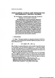
Experiments • CalTech 256 image dataset • Corel image database • CalTech 101 - Face Easy dataset
CalTech 256
p(η ∗ |λ) Inverse Normal Wishart prior on mixture components (conjugate of the multivariate Gaussian distribution)
Kernel PCA + spatial pyramid match kernel single image = 20 dimensional vector
Corel dataset vector quantization 7x7 patches 30,000 data points
• •
Kurihara’s accelerated inference reaches memory limit Incremental algorithm processes data in 4 hours
CalTech101
results
clumps
baseline
30%
100%
References Gomes, Welling, Perona. Incremental Learning of Nonparameteric Bayesian Mixture Models. CVPR 2008. Gomes, Welling, Perona. Memory Bounded Inference in Topic Models. ICML 2008. Blei and Jordan. Variational Inference for Dirichlet Process Mixtures. Journal of Bayesian Analysis 2006 Kurihara, Welling,Vlassis. Accelerated Variational Dirichlet Process Mixtures. ICML 2006
Gamma distribution
Beta distribution
Dirichlet distribution