Incremental On-Line Topological Map Learning for A Visual Homing Application Elvina Motard, Bogdan Raducanu, Viviane Cadenat and Jordi Vitri`a Abstract— In this paper we propose an on-line incremental vision-based topological map learning for AIBO robots. The topological map is represented through a graph, where the vertices encode views from the robot’s environment and the edges the spatial relationship between these views. The views are represented through their SIFT keypoints. The proposed map learning method has been successfully applied to a homing application. Index Terms- topological maps, visual SLAM, AIBO
I. INTRODUCTION Navigation is one of the basic tasks an autonomous robot must be able to perform in an unstructured environment. In order to do so, there are two requirements to be met: first, it needs to know its current position (localization) and second, to know how to get from the current position to the destination. This is a well-studied problem in robotics, and is referred as SLAM (Simultaneous Localization And Mapping). It can be solved by creating and maintaining models (maps) of the environment where the robot is supposed to move. Building models of an environment is a very challenging task. There are several factors that put serious limitations in creating an accurate map, both internal and external. The internal ones are represented by sensor noise, odometry errors, perceptual limitation of the sensors (they have a limited range), etc. As external factors we can mention the complexity/dynamics of the environment that surrounds the robot. However, a lot of effort has been dedicated to overcome these limitations. As a result, two main paradigms have been proposed for indoor robot mapping: metric (gridbased) and topological. Metric maps represent environments by a regular grid. Each cell of this grid can contain information about the presence or absence of an obstacle in the area. Successful SLAM results based on metric mapping of large indoor environments obtained using sonars and laser scanners have been reported in [1],[2],[3] and [4]. Vision-based only approaches (using either single or stereo system) have been demonstrated E. Motard is with the IUP Intelligent Systems (Engineering Department), Paul Sabatier University, 118 route de Narbonne, 31062 Toulouse, France
[email protected] B. Raducanu is with the Computer Vision Center, Edifici ”O” - Campus UAB, 08193 Bellaterra (Barcelona), Spain
[email protected] V. Cadenat is with LAAS-CNRS, Paul Sabatier University, 7 Avenue du Colonel Roche, 31077 Toulouse, France
[email protected] J. Vitri`a is with the Computer Vision Center, Edifici ”O” - Campus UAB, and with the Department of Computer Science, Autonomous University of Barcelona (UAB), 08193 Bellaterra (Barcelona), Spain
[email protected] This work is supported by MEC Grant TIN2006-15308-C02, Ministerio de Educaci´on y Ciencia, Spain. Bogdan Raducanu is supported by the Ramon y Cajal research program, Ministerio de Educaci´on y Ciencia, Spain.
successfully in case of smaller (room size) environments [5], [6], [7] and [8]. On the other hand, topological maps are about the representation of spatial relations between environment’s regions. Topological maps have been biologically inspired from animal behavior [9]. Higher vertebrates appear to construct representations (sometimes referred as cognitive maps) which encode spatial relations between relevant locations in their environment. Under this assumption, visual sensing plays a fundamental role. The topological models were induced by visibility regions associated with landmarks characterized by affine invariant (local or global) feature descriptors [10], [11],[12] and [13]. At a more abstract level, a topological map serves as an example of symbols (different places) and connections between them [14]. Both approaches have strengths and weaknesses: metric maps can provide a more accurate and discriminative representation of the environment, but their complexity can suppose a serious drawback for efficient planning; on the other hand, topological maps offer a more compact representation of the space, but it is not able to disambiguate between quasi-similar views. A comparative analysis between metric and topological mapping is beyond the scope of this work, but a very comprehensive survey can be found in [15]. However, there were some research done on integrating the two approaches by taking advantage from ”the best from both worlds” [16]. This paper takes a topological approach on SLAM. We propose an on-line incremental visual map learning for an AIBO robot. In our case, we represent the image through a set of local descriptors (SIFT), which are invariant to scale, rotation, translation and partial to illumination. The choice for this approach is motivated by the particularity of the robot architecture and by the fact that its design concept is biologically inspired (similar approaches have been taken in [17],[18]). AIBO (and its successor Genibo [19]) belongs to a new generation of robots which opened a new area in the robotic fields: social robotics. They are designed specifically to support a richer form of interaction with people, to cohabitate with them and to be part of their everyday life. For this purpose, they are endowed with human-like perception capabilities like: vision, hearing and tact. In consequence, they lack of other sensorial mechanisms (like sonars, laser scanners, etc.) that are common in general-purposes autonomous systems (such as Pioneer for instance). AIBO is no exception from this and its main perceptual capability is represented by a monocular camera. The existence of two infra-red sensors, one on the nose (just
above the camera) and the other one on the chest, are used for obstacle detection at very short range (20-30 cm). With the proposed method for topological map learning, we developed a homing application. Preliminary results obtained so far are very promising and guarantee an ubiquitous dimension for our approach. The paper is structured as follows: next section is dedicated to briefly recall the SIFT keypoints and their properties. In section 3, we describe the algorithm for topological map learning and its implementation for our problem. In section 4 we report some experimental results and finally, section 5, contains our conclusions and guiding lines for future work. II. IMAGE FEATURE EXTRACTION The scale invariant feature descriptor (SIFT) has been introduced by D. Lowe [13]. The SIFT features correspond to highly discriminative image locations which present an increased robustness against changes in scale, orientation and illumination. The candidate features are selected among the local extrema of the difference between two images (at consecutive scales) in a gaussian scale-space. Let be I the input image and Lσ the result of its convolution with a gaussian kernel at scale σ, i.e.: D(x, y) = Lσ+1 (x, y) − Lσ (x, y)
(1)
Lσ (x, y) = (I ∗ Gσ )(x, y)
(2)
Fig. 1. images
Detecting the maxima and minima of the difference of gaussian
where Then the image is down sampled by a factor of 2 to produce the next level (called octave) in an image pyramid. This is repeated until the image size is so small that it is impossible to detect interest points. The candidate points are searched for in the set: S = Emin {D} ∪ Emin {D}
(3)
where Emin {D} and Emax {D} represent the set of local minima and maxima, respectively, calculated by comparing a center pixel with its eight neighbors at its own scale and the nine neighbors at the scale above and below (see figure 1). In the next stage, the local extrema with low contrast or poor localization are discarded. The keypoint descriptor is then formed by computing local orientation histograms (with 8 bin resolution) for each element of a 4x4 grid overlayed over 16x16 neighborhood of the point. This yields 128 dimensional feature vector which is normalized to unit length in order to reduce the sensitivity to image contrast and brightness changes in the matching stage. A match between two interest points is calculated by the squared distance between them and a similarity criteria is calculated as the ratio between the best and second best match. The similarity measure is used for selection of unique interest points, i.e. a large distance between the best and second best match. Note that the detected SIFT features correspond to distinguishable image regions and include both point features as well as regions along line segments. An example of keypoints matching is showing in figure 2.
Fig. 2. Visual representation of correspondences between keypoints: 178 matches have been found
III. A HOMING APPLICATION A. Problem Description AIBO is a biologically inspired robot. Its behavioral patterns will develop as it learns and grows. It matures through a continuous interaction with the environment and the people it cohabitates with. For this reason, each AIBO is unique. Its human-like behavior is implemented through series of instincts and senses (affective, curiosity, movement instincts and touch, hearing, sight and balance senses). Among them, one of the most crucial for its existence is the ”survival” instinct. Whenever it feels the battery level is below a certain value it starts searching the recharging station. However, some limits are imposed on this built-in behavior: the charging station has to be in the field of view (not occluded by other objects) of the robot and not further than 1 meter. Given this limitation, our approach offers a general capability for the robot to reach the charging station from any given position (and despite of the existence of obstacles). The application block diagram is depicted in figure 3
Fig. 3.
Block diagram of our application
and consists of two parts. The left part corresponds to the incremental map building used for visual SLAM. While its battery is full, the robot is wandering in the environment, learning the map (view graph) of the surroundings. The right part corresponds to the route planning. When the battery level is below a certain threshold, the robot needs to go to recharge. It uses the previous built map in order to find the shortest path to its destination (recharging station). Both aspects will be detailed in the next sections. B. Graph Learning A view graph G = (V, E) is defined as a topological representation consisting of local views (vertices) and their spatial relationship (edges). The local views are represented through the set of associate SIFT features (keypoints): Vk = S(Ik ), where k = 1, 2, ..N represents the vertex index and Ik the corresponding image. Initially, the graph is empty. When a new image Q is acquired (and the number of keypoints is greater than a certain threshold), the algorithm first tries to match this view with any other view in the graph. In other words, we try to find a correspondence between the keypoints of the new image S(Q) and the keypoints of any
of the images previously stored in the graph S(Ik ). This is achieved by choosing the nearest neighbor based on the euclidean distance between two descriptors. The match is then declared as the maximum number of correspondences found: M = max |d(S(Ik ), S(Q))| k
(4)
where |A| represents the cardinality of the set A. If the value of this distance is below a certain threshold (i.e. no match has been found), we connect this new view to the latest recorded view in the graph, E(IN , Q), where N is the current number of views in the graph. Thus, the systems records chains of snapshots, or routes. These routes can be used to find a way back to the start position by homing to each intermediate snapshot in inverted order. The views must be distinguishable, because otherwise the representation could not be used for finding a specific location. Since our map-learning algorithm is exclusively based on visual information, we must guarantee that the recorded views are sufficiently distinct. Additionally, each edge between two vertices P and R has assigned a certain weight E(P, R) =
Fig. 6.
Fig. 4.
AIBO’s energy station and its associated visual pattern
Fig. 5. The five head position used to build the view list and their corresponding snapshots
Correct view matching despite image rotation
invariant to rotation (see figure 6). Each view from this list is matched against each view from the path and each view from which the station can be seen. The next view to be explored and travel to it is chosen in order to guarantee the shortest path to the station. In other words, this corresponds to the edge in the graph (from the matched view list) which has the lowest weight. Once an edge has been followed, its weight is decreased. This, way some edges are reinforced. On the other hand, if an edge is not used, its weight is increased. If it’s value is above a certain threshold, the edge is removed (the associated views are too far apart). IV. EXPERIMENTAL RESULTS
wP R . In this phase, all edges have the same weight, but later on, in the route learning stage, the value of this weight will be updated. C. Route Planning When the robot wants to go the recharging station, it needs to find a path through the graph. The Dijkstra’s algorithm [20] has been used in order to find the shortest path. In our implementation, each view (vertex of the graph) has an associated boolean that allows to know if the energy station is present on this view (thus, we could have several views for the charging station). The robot comes with a built-in functionality to recognize the visual pattern associated to the station pole (see figure 4). During the path finding, all the vertices of the graph are first checked to find all the views from which the station can be seen. Then the possible paths between the current view and the station are calculated. When the last vertex has been reached, it means that AIBO can see the station. In order to travel between the vertices of the view graph we need a homing method. Since the location of a vertex is only encoded in the recorded view, we have to deduce the driving direction from a comparison of the current view to the goal view. For this purpose we first build a list of views that can be seen from AIBO’s head. The list of views is built by dividing AIBO’s hemispheric field of view in 5 regions (with a separation of 45 degrees between them). This is represented in figure 5. When AIBO stands and moves the head, a rolling effect appears. That is due to AIBO’s design. However, this doesn’t represent any problem for us since SIFT keypoints are
The AIBO’s visual system is represented by a web-like, CMOS camera with a maximum resolution of 412x318 pixels. For AIBO programming we used the Remote Framework (RFW) toolkit [21]. It is a C++ library that contains functions to control AIBO based on a client-server architecture over a wireless network between the robot and PC. The main advantage using this toolkit is represented by the fact that all the computation load of the algorithm is executed on PC. For efficiency purposes, the images are transferred from the robot in the JPEG format and decompressed on-the-fly in PC’s memory. This way, we were able to achieve a real-time processing (10 frames/s) at maximum image resolution. For image processing we used OpenCV library. SIFT keypoints were computed using Lowe’s implementation and available on Internet [22]. It is very important to underline here, that in our approach, the train and test phases take place simultaneously. In other words, we don’t create an a priori ’training set’ with images from the robot’s environment. Thus, the initial graph is empty and is incrementally built. A new snapshot is converted in vertex of the graph if it contains at least 50 keypoints. A match between two views in the graph is declared if we can find at leat 10 corresponding keypoints. The initial value of edges’ weight is 100. We increase/decrease this value with a step of 10. The upper threshold to remove an edge is 150. In the figure 7 we represent the evolution of number of connections and vertex of the graph in the route learning stage. After some time, the number of vertices is saturated while the number of edges continues to increase. The interpretation is that after some time, the whole environment was mapped.
Current Vertex 1 2 3 4 5 6 7 8 9 10 11 12 13 14
Fig. 7.
Evolution of the number of vertices and edges of the view graph
As we don’t have any idea of how the environment is (and no information about robot initial position), the strategy for exploration is very simple: we choose a random direction. The different possibilities of movements are thus to turn right, to turn left or to go straight. The only constraint we have regarding the exploration is that the next view that will be seen by the robot after moving has to be connected to the previous one. Thus the movement cannot be too big. We used a fixed turning angle of 50 degrees and a fixed distance of 50 cm. Then the probability to go straight is 66% whereas the one to turn is 33%. These probabilities have been chosen after some tests. The advantage of this strategy is that the environment will be explored without any danger that the agent is caught in an infinite loop. The disadvantage is that the exploration time can be long to get a full map of the environment. In figure 8, we depicted a scenario used to test our approach. The experiment is intended to prove the robustness of our application, in a complex environment, where obstacles are intentionally set between the robot and the station. The upper left image represents the real scenario and the upper right its graphical representation, where the shortest path found by the robot is highlighted. The bottom row corresponds to the views associated with the shortest path found by our robot. The built graph corresponding to this scenario is formed of 21 vertices (views), of which only 4 are enough to find the shortest path. In table I, we depicted some of the vertices of the view graph. (Please note that vertex indexes in this table are not the same with the labels of key views from figure 8). The accuracy of the view matching relies on the SIFT algorithm, which, on its turn depends on the environment conditions and robot position. In general, the matching is very robust (SIFT keypoints are very distinguishable), but sometimes it could happen that we got some false positive (see figure 9). However, the number of mismatched views is low and the system is able to recover from these errors. The view matching could achieve as much as 95% recognition rate. In order to have a good representation of the image,
−→ −→ −→ −→ −→ −→ −→ −→ −→ −→ −→ −→ −→ −→
Connected views 2, 9, 13 (station) 1, 3, 13 2, 10 4 (deadend) 6 5, 7 6, 8, 10, 11 7, 9, 16, 13 8, 1 3, 7 7, 12 11 2, 1, 8 8
TABLE I T OPOLOGICAL REPRESENTATION OF OUR TEST ENVIRONMENT
Fig. 9.
A false positive example
it must have a rich texture. Otherwise, we cannot find a representative number of keypoints. It is the case with regions poor in texture like walls, carpets, furniture, etc. Another source of problems is the presence of similar objects in the environment. In this case, the robot get confused about its position. This means that during the mapping phase, wrong edges will be added between graph nodes. They can be removed afterwards, in the path following phase, because the weight of the edges is updated depending on if the robot can follow the route. If there is a wrong edge and the robot wants to reach the next view following this edge and never finds the next view, then the weight is increased and when it reaches a maximum threshold, it is removed from the graph. Another situation is represented by changes in robot environment (for instance, in the context described above, a box is removed from the scene). If this happens during the mapping phase, the new views of the environment will be added to the graph and new edges will be added between ’old’ and ’new’ views. If this happens during the path following phase, then the robot will try to reach places which are not longer in the environment. The edges linking these views will be increased until they reach a certain threshold and they are removed. Then, new views will be added to the graph (in consequence, new edges will appear) and this way the graph will be updated.
Fig. 8.
The test environment (see text for more details)
V. CONCLUSIONS AND FUTURE WORKS In this paper we proposed a solution for incremental on-line topological map learning for a homing application. Topological maps are inspired from animal behavior and they are a suitable solution for visual SLAM. AIBO is a biologically inspired robot, so we considered this approach is taylored for it. Furthermore, due to its architecture, visual sensing is the only cue it can perceive the environment. The incremental map building provides a ubiquitous dimension of our approach, since no a priori training and knowledge of the environment is required. The views are represented through SIFT keypoints, which are invariant to scale, rotation and changes in illumination conditions. The proposed method was used for a homing application, which proved that AIBO is able to reach the recharging station even when it is far away or its view occluded by obstacles. The experimental results so far are very encouraging, but they are conditioned by the presence of distinct objects presenting a rich texture. In the future we plan to carry out more extensive experiments in larger areas in order to confirm its robustness. Since the graph used here is a deterministic one, we also plan to implement a stochastic version of it (where the transitions are represented by probabilities) and to draw a comparison between the two methods. We would also like to test other feature representation for images and to compare with SIFT. R EFERENCES [1] F. Bourgault, A. A. Makarenko, and S. B. Williams, ”Information Based Adaptive Robotic Exploration”, in Proc. of Intl. Conf. on InteIligent Robots and Systems, vol.1, pp. 540-545, Switzerland, 2002 [2] M. Montemerlo and S. Thrun, ”Simultaneous Localization and Mapping with Unknown Data Association Using FastSLAM”, in Proc. of Intl. Conf. on Robotics and Automation, vol. 2, pp. 1985-1991, Taiwan, 2003 [3] A. I. Eliazar and R. Parr, ”DP-slam 2.0”, in Proc. of Intl. Conf. on Robotics and Automation, vol. 2. pp.1314-1320, EE.UU, 2004 [4] A. Diosi and L. Kleeman, ”Advanced Sonar and Laser Range Finder Fusion for Simultaneous Localization and Mapping”, in Proc. of Intl. Conf. on InteIligent Robots and Systems, vol. 2, pp. 1854-1859, Japan, 2004
[5] S. Se, D. Lowe, and J. Little, ”Mobile Robot Localization and Mapping with Uncertainty Using Scale Invariant Visual Landmarks,” in International Journal of Robotics Research, vol. 21, no. 8, pp. 735758, 2002 [6] M. G. P. Rybski, S. Roumeliotis and N. Papanikopoulous, ”Appearance Based Minimalistic Metric SLAM,” in Proc. of Intl. Conf. on Intelligent Robots and Systems, vol.1, pp. 194–199, USA, 2003 [7] R. Sim, P. Elinas, M. Griffin and J. J. Little, ”Vision-based SLAM using the Rao-Blackwellised Particle Filter”, in Proc. of IJCAI Workshop Reasoning with Uncertainty in Robotics, pp. n/a, UK, 2005 [8] N. Karlsson, E. Di Bernardo, J. Ostrowski, L. Goncalves, P. Pirjanian and M. E. Munich, ”The vSLAM Algorithm for Robust Localization and Mapping”, in Proc. of Intl. Conf. on Robotics and Automation, vol.1, pp. 24-29, Spain, 2005 [9] T.J. Prescott, ”Spatial Representation for Navigation in Animals”, in Adaptive Behaviour, vol. 4, no.2, pp.n/a, 1996 [10] R. Sims and G. Dudek, ”Learning Environmental Features for Pose Estimation”, in Image and Vision Computing, vol. 19, no. 11, pp. 733– 739, 2001 [11] J. Wolf, W. Burgard, and H. Burkhardt, ”Robust Vision Based Localization for Mobile Robots Using Image-Based Retrieval System Based on Invariant Features,” in Proc. of Intl. Conf. on Robotics and Automation, vol.1, pp. 359-365, Taiwan, 2003 [12] Z. Lin, S. Kim and I.S. Kweon, ”Recognition-based Indoor Topological Navigation Using Robust Invariant Features”, in Proc. of Intl. Conf. on Intelligent Robots and Systems, pp. 3975-3980, Canada, 2005 [13] D. G. Lowe, ”Distinctive Image Features from Scale-Invariant Keypoints,” in International Journal of Computer Vision, vol. 60, no. 2, pp. 91-110, 2004 [14] B. Kuipers and Y. T. Byan, ”A Robot Exploration and Mapping Strategy Based on a Semantic Hierarchy of Spatial Representations,” in Journal of Robotics and Autonomous Systems, vol. 8, pp. 47-63, 1991 [15] S. Thrun, ”Learning Maps for Indoor Mobile Robot Navigation”, in Artificial Intelligence, vol. 99, no.1, pp. 21-71, 1998 [16] S. Thrun, J.-S- Gutmann, D. Fox, W. Burgard, B.J. Kuipers, ”Integrating Topological and Metric Maps for Mobile Robot Navigation: A Statistical Approach”, in Proc. of the AAAI Fifteenth National Conference on Artificial Intelligence, pp.n/a, USA, 1998 [17] M.O. Franz, B. Schlkopf, H.A. Mallot and H.H. Blthoff, ”Learning View Graphs for Robot Navigation”, in Autonomous Robots, vol.5, no.1, pp. 111-125, 1998 [18] N. Cuperlier, M. Quoy, P. Gaussier, C. Giovanangelli, ”Navigation and planning in an unknown environment using vision and a cognitive map”, in Proc. of IJCAI Workshop Reasoning with Uncertainty in Robotics, pp. n/a, UK, 2005 [19] Genibo Pet Robot, http://www.dasatech.com [20] T. H. Cormen, C. E. Leiserson, R. L. Rivest, and C. Stein, ”Introduction to Algorithms”, in MIT Press, 2001 [21] AIBO Remote Framework (RFW), http://openr.aibo.com [22] SIFT algorithm, http://www.cs.ubc.ca/ lowe/keypoints/