Indexing Uncertain Data
∗
Pankaj K. Agarwal
Siu-Wing Cheng
Yufei Tao
Duke University Durham, NC, USA
[email protected]
HKUST Hong Kong, China
[email protected]
CUHK Hong Kong, China
[email protected]
Ke Yi HKUST Hong Kong, China
[email protected]
ABSTRACT
Keywords
Querying uncertain data has emerged as an important problem in data management due to the imprecise nature of many measurement data. In this paper we study answering range queries over uncertain data. Specifically, we are given a collection P of n points in R, each represented by its one-dimensional probability density function (pdf). The goal is to build an index on P such that given a query interval I and a probability threshold τ , we can quickly report all points of P that lie in I with probability at least τ . We present various indexing schemes with linear or near-linear space and logarithmic query time. Our schemes support pdf’s that are either histograms or more complex ones such as Gaussian or piecewise algebraic. They also extend to the external memory model in which the goal is to minimize the number of disk accesses when querying the index.
Indexing, uncertain data, range query
Categories and Subject Descriptors F.2 [Analysis of algorithms and problem complexity]: Nonnumerical algorithms and problems; H.3.1 [Information storage and retrieval]: Content analysis and indexing— indexing methods
General Terms Algorithms, theory ∗ P.
K. Agawal is supported by NSF under grants CNS-05-40347, CFF-06-35000, and DEB-04-25465, by ARO grants W911NF07-1-0376 and W911NF-08-1-0452, by the NIH grant 1P50-GM08183-01, and by a grant from the US-Israel Binational Science Foundation; S.-W. Cheng is supported by HKRGC under grant GRF 612107; Y. Tao is supported by HKRGC under grants GRF 1202/06, GRF 4161/07, and GRF 4173/08; and K. Yi is supported by Hong Kong Direct Allocation Grant (DAG07/08).
Permission to make digital or hard copies of all or part of this work for personal or classroom use is granted without fee provided that copies are not made or distributed for profit or commercial advantage and that copies bear this notice and the full citation on the first page. To copy otherwise, to republish, to post on servers or to redistribute to lists, requires prior specific permission and/or a fee. PODS’09, June 29–July 2, 2009, Providence, Rhode Island, USA. Copyright 2009 ACM 978-1-60558-553-6 /09/06 ...$5.00.
1. INTRODUCTION Indexing a set of points for answering range queries is one of the most widely studied topics in spatial databases [21] and computational geometry [3], with a wide range of applications. Most of the work to date deals with certain data, that is, the points have exact coordinates and the goal is to index them so that all points inside a query range can be reported efficiently. Recent years have witnessed a dramatically increasing amount of attention devoted to managing uncertain data, due to the observation that many realworld measurements are inherently accompanied with uncertainty [7, 14, 16, 23, 24]. Depending on the application, there are two models of data uncertainty, which we describe in the context of range searching. In the tuple-level uncertainty model (also known as existentially uncertain data) [7, 16, 25], a point in the data set still has a precise position but its existence is uncertain. Usually it is assumed that each point appears with some probability and all the points are independent. We could relax the independence assumption and introduce “rules” to model the correlation between the points. In the attributelevel uncertainty model [14, 23, 24], a point always exists but its location is uncertain, and is modeled as a probability distribution over space. Again we usually assume the points are independent but it is not necessary. The generally agreed semantics for querying uncertain data is the thresholding approach [14, 16], i.e., for a particular threshold τ , retrieve all the tuples that appear in the query range with probability at least τ . Under the tuple-level uncertainty model, a d-dimensional range searching problem over uncertain data simply becomes a (d + 1)dimensional range searching problem over certain data, by treating the probability as another dimension. The same observation has also been made in [25]. The independence assumption is irrelevant since each point is considered individually. Of interests is the attribute-level uncertainty model, where each point has a pdf, and we wish to report all points whose probability of being inside the query range is at least τ . This problem is nontrivial, even in one dimension, as it cannot be easily transformed to an instance of range searching on certain data. The na¨ıve approach of examining each point one by one and computing its proba-
bility of being inside the query is obviously very expensive. In this uncertainty model, the independence assumption is again irrelevant with respect to range queries. Problem definition. Let P = {p1 , . . . , pn } be a set of n uncertain points in R, where each pi is specified by its probability density function (pdf) fi : R → R+ ∪ {0}. We assume that each fi is a piecewise-uniform function, i.e., a histogram, consisting of at most s pieces for some integer s ≥ 1. In practice, such a histogram can be used to approximate any pdf with arbitrary precision. In some applications each point pi has a discrete pdf, namely, it could appear at one of a few locations, each with a certain probability. This case can also be represented by the histogram model using infinitesimal pieces around these locations, so the histogram model also incorporates the discrete pdf case. We will adopt the histogram model by default throughout the paper. For simplicity, we assume s to be a constant for most of the discussion. Some of our indexes also support more complicated pdf’s (such as Gaussian or piecewise algebraic), and we will explicitly say so for these indexes. Given the set P and the associated pdf’s, the goal is to build an index on them so that for a query interval I and a threshold τ , all points p such that Pr[p ∈ I] ≥ τ are reported efficiently. We also consider the version where τ is fixed in advance. We refer to the former as the variable threshold version and the latter as the fixed threshold version of the problem. The latter version is useful since in many applications the threshold is always fixed at, say, 0.5. Moreover, the user can often tolerate some error ε in the probability. In this case we can build 1/ε fixed-threshold indexes with τ = ε, 2ε, . . . , 1, so that a query with any threshold can be answered with error at most ε. Applications. The problem of range searching over uncertain data was first introduced by Cheng et al. [14] and has numerous applications in practice. For example, in a sensor network, a certain measurement, say temperature, of a location may be taken by multiple sensors. Due to various imprecision factors, the readings of these sensors may not be necessarily identical, in which case the temperature of the location can be conveniently modeled as a pdf. In this context, a query in our problem would retrieve “all the locations whose temperatures are between 100 and 120 degrees with probability at least 50%”. It is not hard to see that there are many similar scenarios involving uncertain data. In fact, our problem is also important even in several traditional applications where no uncertainty seems to exist. For instance, consider a movie rating system (such as the one at Amazon) where each reviewer can give a rating from 1 to 10. A query of our problem would find “all the movies such that at least 90% of the ratings it receives are at least 8”. Previous results. Cheng et al. [14] considered the above problem in a simpler form, namely, where each fi (x) is a uniform distribution — a special case of our definition in which the histogram consists of only one piece. For the fixed-threshold version with threshold 0 < τ ≤ 1, they proposed an index of O(nτ −1 ) size with O(τ −1 log n + k) query time, where k is the output size. These bounds depend on τ −1 , which can be arbitrarily large. This index also does not extend to histograms consisting of two or more pieces. They presented heuristics for the variable threshold version without any performance guarantees. Tao et al. [23, 24]
considered the problem in two and higher dimensions, and presented some index structures based on space partitioning heuristics. They prune points whose probability of being inside the query range is either too low or too high, but the query procedure visits all points of P in the worst case. Finally, yet another heuristic is presented in [19], but it is still the same as a sequential scan in the worst case. Cheng et al. [14] also showed that the fixed-threshold version of the problem is at least as difficult as 2D halfplane range reporting (i.e., report all points lying in a query halfplane), and that it can be reduced to 2D simplex queries (report all points lying in a query triangle). However the complexities of these two problems differ significantly: With linear space, a halfplane range-reporting query can be√answered in time Θ(log n+k) [12], while the latter takes Ω( n) time [13]. So there is a significant gap between the current upper and lower bounds for range searching over uncertain data. Also related is the work by Singh et al. [22], who considered the problem of indexing uncertain data that are categorical, namely, each random object takes a value from a discrete, unordered domain. The index structures presented there are again heuristic solutions. Our results. In this paper, we make a significant theoretical step towards understanding the complexity of indexing uncertain data for range queries. We present linear or nearlinear size indexing schemes for both the fixed and variable threshold versions of the problem, with logarithmic or polylogarithmic query times. Specifically, we obtain the following results. For the fixed-threshold version, we present a linear-size index that answers a query in O(log n + k) time (Section 2). These bounds are clearly optimal (in the comparison model of computation). We first show that this problem can be reduced to a so-called segments-below-point problem: indexing a set of segments in R2 so that all segments lying below a query point can be reported quickly. Then we present an optimal index for the segments-below-point problem — a linear-size index with O(log n + k) query time. This result shows that the fixed-threshold version has exactly the same complexity as the halfplane range-reporting problem, closing the large gap left in [14]. In Section 3 we present a simpler index of size O(nα(n) log n) and query time O(log n + k). This index extends to more general pdf’s, such as Gaussian distributions or other piecewise algebraic pdf’s, and they can also be used to approximately count the number of uncertain points lying in the query interval. For the variable-threshold version, we use a different reduction and show that it can be solved by carefully indexing a number of points in R3 for answering halfspace range queries. Combining with the very recent result of Afshani and Chan [1] for 3D halfspace range reporting, we obtain an index for the variable-threshold version of our problem with O(n log2 n) space and O(log 3 n + k) query time (Section 4). Although the bounds have extra log factors in this case, our result shows that this problem is still significantly easier than 2D simplex queries. Finally, we show that our indexing schemes can be dynamized, supporting insertions and deletions of (uncertain) points with a slight increase in the query time. If the resulting index needs to be stored on disk, the query time is dominated by the number of I/Os (or page reads), where
g(x) e f (x)
F (x)
(xl , xr )
d c
b a
b
c xl
(i)
d e xr
x
a
b
c
d
x
e
a
b
(ii)
c
d
e
x
(iii)
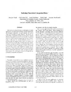
Figure 1. Reduction to the segments-below-point problem: (i) pdf, (ii) cdf, and (iii) threshold function. 6
each I/O reads a whole disk block of size B. We also show how to externalize our index so that the queries can be answered in an I/O-efficient manner.
2.
4
FIXED-THRESHOLD RANGE QUERIES
We present an optimal index for answering range queries on uncertain data where the probability threshold τ is fixed. Our index uses linear space and answers a query in the optimal O(log n + k) time. These bounds do not depend on the particular value of τ . We first describe in Section 2.1 the reduction to the segments-below-point problem. Next we describe three indexing schemes for the latter problem, each of which reduces a segments-below-point query to answering halfplane range-reporting queries. The first index, based on the√segment tree, uses linear space and answers a query in O( n + k) time (Section 2.3). The second one, based on the interval tree, uses O(n log n) space and answers a query in O(log n + k) time (Section 2.4). We then combine them to construct an index of linear size with O(log n + k) query time (Section 2.5). We conclude this section by describing how we make the index dynamic and extend it to the I/O model.
2.1 A geometric reduction Let p be an uncertain point in R, and let f : R → R be its pdf. Suppose the histogram of f consists of s pieces, and let f (x) = yi ,
for xi−1 ≤ x < xi , i = 1, . . . , s.
We set x0 = −∞, xs = ∞, and y1 = ys = 0; see Fig1 (i). The cumulative distribution function (cdf) F (x) = Rure x f (t)dt is a monotone piecewise-linear function consist−∞ ing of s pieces; see Figure 1 (ii). Let the query range be [xl , xr ]. The probability of p falling inside [xl , xr ] is F (xr ) − F (xl ). We define a function g : R → R, which we refer to as the threshold function. For a given a ∈ R, let g(a) be the minimum value b such that F (b) − F (a) ≥ τ . If no such b exists, g(a) is set to ∞; see Figure 1 (iii). Lemma 1. The function g(x) is non-decreasing and piecewise linear consisting of at most 2s pieces. Proof. Suppose we continuously vary x from −∞ to ∞. For x = −∞, g(x) = min{y | F (y) = τ }; g(x) stays the same until x reaches x1 . As we increase x further, g(x) increases linearly, with the slope depending on the pieces of the histogram f that contain x and g(x). When either x or g(x) passes through one of the xi ’s, the slope changes. There are at most 2(s − 1) such changes; see Figure 1. Given the description of the pdf f , the function g can be constructed easily. Once we have the threshold function g,
7
5
3 2 1
Figure 2. The indexing scheme for a set of lines: thick polygonal chain is the lower envelope of S; L1 (S) = {1, 2, 6}, L2 (S) = {3, 7}, L3 (S) = {4, 5}.
the condition Pr[p ∈ [xl , xr ]] ≥ τ simply becomes checking whether xr ≥ g(xl ). Geometrically, this is equivalent to testing whether the point (xl , xr ) ∈ R2 lies above the polygonal line representing the graph of g (see Figure 1). We construct the threshold function gp for each point p in P . Let S be the set of at most 2ns segments in R2 that form the pieces of these n functions; S can be constructed in O(n) time. We label each segment of gp with p. The problem of reporting the points of P that lie in the interval [xl , xr ] with probability at least τ becomes reporting the segments of S that lie below the point (xl , xr ) ∈ R2 : If the procedure returns a segment labeled with p, we return the point p. Each polygonal line being x-monotone, no point is reported more than once. We thus have the following problem at hand: Let S be a set of n segments in R2 . Construct an index on S so that for a query point q ∈ R2 , the set of segments in S lying directly below q, denoted by S[q], can be reported efficiently. For simplicity, we assume the coordinates of the endpoints of S to be distinct; this assumption can be removed using standard techniques. We call this problem the segmentsbelow-point problem.
2.2 Half-plane range reporting We begin by describing an index for the special case when all segments in S are full lines and we want to report the lines of S lying below a query point. This problem is dual to the well-known half-plane range reporting problem, for which there is an O(n)-size index with O(log n + k)-time [12]. We briefly describe a variant of this index (in the dual setting), denoted by H(S), which we will use as a building block. If we view each line ℓ in S as a linear function ℓ : R → R, then the lower envelope of S is the graph of the function ES (x) = minℓ∈S ℓ(x), i.e., it is the boundary of the unbounded region in the planar map induced by S that lies below all the lines of S (see Figure 2). We represent the lower
v
v1
v2
σ1
σ2 3m
1ℓ
v3
σ3 σv 1r
v4
σ4
v5
σ5
2r
2m 2ℓ
3r
Figure 3. A segment tree node with fanout r = 5.
envelope as a sequence x0 = −∞, ℓ1 , x1 , ℓ2 , . . . , ℓr , xr = +∞, where the xi ’s are the x-coordinates of the vertices of the lower envelope, and ℓi is the line that appears on the lower envelope in the interval [xi−1 , xi ]. Note that the lines appear along the envelope in decreasing order of their slopes. We partition S into a sequence L1 (S), L2 (S), . . ., of subsets, called layers. L1 (S) ⊆ S consists of the lines that appear on the lower envelope of S. For i > 1, Li (S) is the set of lines S that appear on the lower envelope of S \ i−1 j=1 Lj (S); see Figure 2. For each i, we store the aforementioned representation of layer Li (S) in a list. To answer a query q = (qx , qy ), we start from L1 (S) and locate the interval [xi−1 , xi ] that contains qx , using binary search. Next we walk along the envelope of L1 (S) in both directions, starting from ℓi , to report the lines lying below q, in time linear to the output size. Then we query the rest of the layers L2 (S), L3 (S), . . . in order until no lines have been reported at a certain layer. By using fractional cascading [11] on the x-coordinates of the envelopes of these layers, the total query time can be improved to O(k) plus the initial binary search in L1 (S). The size of the index is linear, and it can be constructed in O(n log n) time [12]. The statement below is slightly more general than that appeared in [12]. Lemma 2. Let S be a set of n lines in the plane. We can construct in O(n log n) time an index on S of linear size, so that given a query point q ∈ R2 and any line in L1 (S) below q, all k lines of S lying below q can be reported in O(k) time.
2.3 Segment-tree based index This subsection describes an index for the segments-belowpoint problem, based on the segment tree, that uses linear √ space and answers a query in O( n + k) time. We later (cf. Section 2.5) bootstrap this index to improve the query time to O(log n + k) while keeping the size linear. We fix a parameter r and construct a segment tree T of fanout r — an r-ary tree that defines an r-way hierarchical decomposition of the plane into vertical slabs, each associated with a node of T. Let σv denote the slab corresponding to a node v. The slabs associated with the children of v are defined as follows. We partition σv into r vertical sub-slabs σ1 , . . . , σr , each containing roughly the same number of endpoints of segments in S. We create r children v1 , . . . , vr of v and associate σi with vi ; see Figure 3. A node v is a leaf if σv does not contain any endpoint of S in its interior. We call any number of contiguous sub-slabs a multi-slab
at v. Let σv [i : j] = σi ∪ · · · ∪ σj denote the multi-slab at v spanned by sub-slabs σi , . . . , σj . Obviously there are O(r 2 ) multi-slabs at any v. For any segment s, consider the highest node v where it intersects two or more sub-slabs. At v we partition s into up to three pieces: a middle piece sm that spans the maximal multi-slab at v, a left piece sl , and a right piece sr . More precisely, if s spans slabs σi , . . . , σj , then sm = s ∩ σv [i : j], and it is associated with the multislab σv [i : j]. If the left endpoint of s lies in the interior of σi−1 , then sl = s ∩ σvi−1 , and if the right endpoint of s lies in the interior of σvj+1 , then we set sr = s ∩ σvj+1 . See Figure 3. Next, we recursively partition the left and right pieces of s following the r-ary tree. A segment is thus partitioned into at most three pieces at any level of the tree, resulting in a total of O(logr n) pieces. Note that each piece ends up with spanning a multi-slab at some node. Let Svi:j denote the set of segments associated with the multi-slab σv [i : j] at v, and let Hvi:j denote the full lines containing these segments. We the index on Hvi:j deP build scribed in Section 2.2. Since |Svi:j | = O(n logr n) and the index built for each multi-slab has linear size, the size of the overall index is also O(n logr n), and it can be constructed in O(n logr n log n) time. To report the segments of S lying below a query point q, we visit all the nodes v of T such that q ∈ σv . At each v, we query the index corresponding to all the multi-slabs that contain q. Overall we query a total of O(r 2 logr n) multi-slabs, so the total query time is O(r 2 logr n log n + k). √ Choosing r = n1/4 / log n gives us the following. Lemma 3. Let S be a set of segments in the plane. We can construct in O(n log n) time an index of linear size on S so that all segments of S lying below a query point can be √ reported in O( n + k) time. Remark. The query time of the above scheme can be improved to√O(nε + k) for any small constant ε, but a query time of O( n + k) is all we need for the bootstrapping later. By choosing r = 2, we can construct an indexing scheme of size O(n log n) with query time O(log2 n + k). Using fractional cascading the query time can be improved to O(log n + k).
2.4 Interval-tree based index We now describe a different index to store S, based on the interval tree, that uses O(n log n) space and answers a query in time O(log n + k). An interval tree T for S is built as follows. Let E be the set of endpoints of the segments of S. We first choose the median of E, and vertically divide the plane into two halves. We store this splitting line at the root of T and then build its two subtrees for the two halves recursively. Similar to the segment tree, the interval tree T also hierarchically partitions the plane into O(n) canonical vertical slabs. For a node u ∈ T, let σu be the slab associated with u and xu the x-coordinate of the splitting line at u. For the root u of T, σu is the entire plane. For each u with children v and w, xu is the median of the x-coordinates of E ∩ σv , and the line x = xu partitions σu into σv and σw . When |E ∩ σu | = 1, we stop the partitioning and make u a leaf. For a node u, let p(u), Sb(u), l(u), and r(u) denote the parent, sibling, left child, and right child of u, respectively. A segment s ∈ S is now stored at the highest node u such that the splitting line x = xu intersects s. Let Su ⊆ S be the set of segments stored at u. Since each segment only appears
P in one Su , u |Su | = O(n). Each segment s ∈ Su is split by + x = xu into a left segment s− and a right segment S s− . Let − − + + − Su = S {s | s ∈ Su }, Su = {s | s ∈ Su }, S = u Su , and S + = u Su+ . Note that for any segment s ∈ Su and for any point q 6= xu lying above s, either s− or s+ lies below q, but not both. Therefore it suffices to build separate indexing schemes for S − and S + and report S − [q] and S + [q] for a query point q. We describe the indexing scheme for S − ; a similar scheme works for S + . It is tempting to construct an indexing scheme on Su− at each node as in a standard interval tree. However, the segments in Su− do not span the slab σl(u) , so we cannot regard them as a set of lines and build the indexing scheme described of Section 2.2. Instead we refine the sets Su− and proceed as follows. xc
xb
xa 1
2
a
3
u. Let w be the leaf of T such that p, the left endpoint of e lies in σw . If w = z, then e ∈ Φz and there is nothing to prove. So assume that w 6= z, and let v be the lowest common ancestor of w and z. Then q ∈ σr(v) , and p ∈ σl(v) . Since e lies below q, e intersects σr(v) and thus crosses the line x = xv . Therefore u is a proper ancestor of v, implying that e ∈ Sul(v) and e ∈ Φl(v) . This completes the proof of the lemma. In view of the above lemma, we can answer a query for a point q as follows: We visit Πq in a top-down manner. Suppose we are at a node v. If v is leaf, we report the (at most one) segment in Φv provided it lies below q. If v is an internal node and r(v) ∈ Πq , then we query the index on Hl(v) with q and report all segments of Φl(v) [q]. Since we query the indexing scheme at O(log n) nodes, the overall query time is O(log2 n + k) time. Again, using the fractional cascading on the indexing schemes built at each node of T, the query time can be reduced to O(log n + k). Hence, we obtain the following.
b 6
c
4 7 σe
Lemma 5. Let S be a set of segments in the plane. We can construct in O(n log2 n) time an index of O(n log n) size on S so that all segments of S lying below a query point can be reported in O(log n + k) time.
5 e
σd
d
σc
2.5 Hybrid index
σb
Figure 4. The Φv and Suv ’s for a set of 7 segments for (a portion of) the interval tree on the right: Sab = {1, 2, 5, 7}, Sac = {1, 2, 7}, Sad = {1}, Sae = {2, 7}, Sbd = {4}, Sbe = {6}; Φc = {1, 2, 7}, Φe = {2, 6, 7}.
For a proper descendant v of a node u, we define Suv ⊆ Su to be Suv = {s ∈ Su− | s’s left endpoint ∈ σv }.
(1)
Note that by definition, Suv is empty if v is in the right subtree of u. For a node v, let [ Suv , (2) Φv = u
where the union is taken over all proper ancestors of p(v). See Figure 4 for an example. For a fixed v, the sets Suv are pairwise disjoint; while for a fixed u, the sets S Puv induce a binary hierarchical partitioning of Su . Hence, u,v |Suv | = O(n log n). A crucial observation is that if v is the left child of its parent, then each segment in Φv spans the slab σSb(v) . Hence, a point q ∈ σSb(v) lies above a segment e of Φv if and only if it lies above the line containing e. Let Hv be the set of lines containing the segments in Φv . At each node v, we construct the index on Hv described in Section 2.2. The total size of the overall indexing scheme is O(n log n), and it can be constructed in time O(n log2 n). The following lemma suggests how to report the segments in S − [q] for a query point q. Let Πq denote the path from the root to the leaf z of T such that q ∈ σz . Lemma 4. Let q be a query point, let z be the leaf of T such that q ∈ σz , and let e ∈ S − be a segment that lies below q. If the left endpoint of e does not lie in σz , i.e., e 6∈ Φz , then there is a node v ∈ Πq such that q ∈ σr(v) and e ∈ Φl(v) .
Proof. Suppose e ∈ Su− , then e ⊆ σl(u) and the right endpoint of e lies on the line x = xu , the splitting line of
We now describe an optimal index for answering segmentsbelow-point queries, by combining the previous two schemes along with additional ideas. We start with the interval-tree based index from the previous subsection. We stop the topdown construction of the interval tree T as soon as there are Θ(log2 n) endpoints of S left in the slab, that is, the “atomic slab” σz for each leaf z of T contains Θ(log2 n) endpoints of S. For each internal node u, we define Su− and Su+ as above, and let S − , S + be as defined earlier. Since we have “fat” leaves, not all segments will be split — those with both endpoints lying in the same atomic slab will not. For a leaf z, let Sz be the set of segments whose both endpoints lie in σz . We build a segment-treePbased index (Lemma 3) on Sz . Since |Sz | = O(log2 n) and z |Sz | ≤ n, a segments-belowpoint query on Sz can be answered in O(log n + k) time and the total size and construction time of the index, summed over all leaves, are linear and O(n log n), respectively. Next we describe the index we build on S − ; a similar index is built on S + . Let Suv , Φv , and Hv be defined as earlier. By Lemma 4, if a segment e ∈ S − lies below a point q ∈ σz for a leaf z ∈ T, then either (i) e ∈ Φz , or (ii) there is an internal node u such that e ∈ Φl(u) and q ∈ σr(u) ; in this case a segment of Φl(u) lies below q if and only if the line containing it lies below q. To handle (i), we build in O(|Φz | log n) time the segment-tree based linear-size index on Φz for each leaf P z. Since the left endpoints of all segments in Φz lie in σz , z |Φz | ≤ n. Therefore the total size of the index over all leaves is O(n), and they can be constructed in O(n log n) time. It thus suffices to describe how we handle case (ii), which is the more interesting case. Let Λ be the set of pairs (u, z) such that z is a leaf and u is proper ancestor of z. For a node v, let Λ(v) ⊆ Λ be the set of pairs (u, z) such that z is a descendant of v and u is a proper ancestor of p(v). Let nuz = |Suz |, and let Huz be the set of lines of containing the segments in Suz . For two pairs (u, z), (u′ z ′ ) ∈ Λ, Suz and Su′ z ′ are disjoint because the left endpoints of all segments in Suz lie in σz and
the right endpoints lie on the splitting line x = xu . Hence, P S n ≤ n. By (2), Φ = uz v (u,z)∈Λ (u,z)∈Λ(v) Suz . Therefore a set Suz is included in Φv at all nodes v that lie on the path from l(u) to z; see Figure 5. To reduce the size of the index to linear, instead of building a separate index for each Φv , we build a more global index. Namely, we build in O(nuz log n) time a linear-size halfplane-range-reporting index (cf. Lemma 2) on Huz , where z is a leaf. By Lemma 2, if we know a line in L1 (Huz ) lying below q, we can report Huz [q] in time proportional to its size. Returning to the problem of reporting Φv [q] for a point q ∈ σSb(v) , we now need an index that returns one representative line of L1 (Huz ) lying below q (if there exists one), for each pair (u, z) ∈ Λ(v). We can then use the index built on Huz to report the remaining lines S in Huz [q]. One possibility is to build an index on the set (u,z)∈Λ(v) L1 (Huz ) at each node to find such a line, but |L1 (Huz )| = |Huz | in the worst case, so this will again lead to an index of size O(n log n). The following observation will help us in reducing the size. xc
xb
xa a
5 4 b
3 2
f
c
1 σe
σd
σf
e
d
σc σb
Figure 5. Set Sae = {1, 2, 3, 4, 5} and the strip Σae (shaded); Sae is included in Φe (queried in slab σd ) and Φc (queried in Φf ); e = {1, 2, 3} and H c = {3, 4, 5}. Hae ae
For a node v, Φv is queried by a point q only when v is the left child of p(v) and q ∈ σSb(v) . Let V denote the set of nodes v ∈ T such that v is left child of p(v). Let Σuz be the strip formed by the splitting line at u and the right boundary of σz ; see Figure 5. The right endpoint of each segment in Suz lies on the right edge of Σuz and the left endpoint lies to the left of Σuz , so each segment spans Σuz . Let w1 , w2 , . . . , wr be the nodes such that each wi is the right child of p(wi ) and p(wi ) lies on the path from l(u) to z; the (left) sibling of each wi also lies on this path. The slabs σw1 , . . . , σwr induce a partitioning of Σuz . Suz (or rather Huz ) is queried only by the points lying in σwi , for 1 ≤ i ≤ r. For a query point q ∈ σwi , we need to report one (representative) line of Huz lying below q. We choose the representative lines of Huz as follows. For a node v on the path from l(u) to z such that v ∈ V ((u, z) ∈ Λ(v) and v Sb(v) is one of the wi ’s), we define Huz ⊆ Huz to be the set of lines that appear on the lower envelope of Huz within v σSb(v) ; set nvuz = |Huz |. If nvuz ≥ 2, then at most one line of v Huz will appear on the lower envelope of Huz on the right e side of σSb(v) (for example, only line 3 of Hae may appear on the lower envelope of Hae on the right side of σd ). Since r = O(log n), we have X nvuz = nuz + O(log n). v∈V,(u,z)∈Λ(v)
v For a pair u, z, the sets Huz can be computed in O(nuz log n)
v time by constructing the lower envelope of Huz . Huz is the set of representative lines that are stored at v. S v For a node v ∈ V, let Γv = (u,z)∈Λ(v) Huz be all the representative lines stored at v. We build in O(|Γv | log n) time the halfplane-range-reporting index of linear size on Γv . For each line ℓ in Γv , we store a pointer to its copy in Huz . Finally, we also build a fractional-cascading structure on these indexing schemes. Summing over all nodes v ∈ T, X X X nvuz |Γv | = v∈V
v∈V (u,z)∈Λ(v)
=
X
X
nvuz
(u,z)∈Λ v∈V,(u,z)∈Λ(v)
=
X
(nuz + O(log n))
(u,z)∈Λ
= O(n) + O = O(n).
„
« n log n log n log2 n
This completes the description of the index we build. Putting all the pieces together, the total size of the index is O(n), and it can be constructed in O(n log n) time. For a query point q, the set S[q] is reported as follows. We first find in O(log n) time the leaf z whose slab contains q. Next, we report in O(log n+|Sz [q]|) time the set Sz [q]. Then, we report S − [q] using Lemma 4: We first query the index on Φz and report in O(log n + |Φz [q]|) time the set Φz [q]. Next, for each node v ∈ Πq , if v is the right child of p(v), we report the set HSb(v) [q]. We accomplish this in two stages: We first query the index on ΓSb(v) and report in O(|ΓSb(v) [q]|) time the set ΓSb(v) [q], i.e., the set of representative lines of HSb(v) that lie below q. Let ℓ ∈ ΓSb(v) [q] be the line that belongs to Huz . We then report the set Huz [q] in time proportional to its size by querying the index built on Huz . The total time spent at v is O(|HSb(v) [q]|). We spend an additional O(log n) time at the root of T to search in the fractional cascading structure built on top of Γv ’s. Finally, we report S + [q] in a similar manner. Putting everything together, the total query time is O(log n + |S[q]|). Theorem 6. Let S be a set of n segments in R2 . We can build in O(n log n) time a linear-size index on S so that all k segments of S lying below a query point can be reported in O(log n + k) time. Since each uncertain point produces O(s) segments in the segments-below-point problem, we immediately have the following. Corollary 7. Given a set P of n uncertain points in R1 , each associated with a histogram having s pieces, and a threshold parameter 0 < τ ≤ 1, we can build in O(n log n) time a linear-size index on P so that a range query on S with probability threshold τ can be answered in O(log n + k) time, where k is the output size.
2.6 Extensions Finally, we briefly describe two useful extensions of our indexing scheme. Externalization. It is not difficult to externalize our index under the standard two-level I/O model [6], so that the query can be answered I/O-efficiently. Agarwal et al. [2]
developed an external index for half-plane range reporting. Although not explicitly mentioned in [2], their structure is amenable to fractional cascading, so that we can extend Lemma 2 to the I/O model, namely, given any line in L1 (S) below a query point q, all the k lines in S lying below q can be reported in O(k/B) I/Os using an index occupying O(n/B) disk blocks. Next we externalize the segment-tree based index. The p fanout of the segment tree is set to r = (n/B)1/4 / log(n/B), and the leaf size of the tree is set to Θ(B). For each multislab, we build the external half-plane range-reporting index for its segments, as mentioned above. The height of the tree is still O(1), and it takes O(r 2 +k/B) I/Os to answer a query. So we obtain a linear-size index for S so thatpall segments below a query point can be reported using O( n/B + k/B) I/Os. Equipped with these schemes, we can go through the construction of the hybrid index, while only changing the leaf size from Θ(log2 n) to Θ(B log2 n). Without repeating the tedious details, we conclude with the following. Theorem 8. Given a set P of n uncertain points in R, their pdf ’s, each of which is a histogram of constant size, and a parameter 0 < τ ≤ 1, we can build a linear-size externalmemory index on S such that a range query with probability threshold τ can be answered in O(log n + k/B) I/Os. Dynamization. Finally we briefly discuss how to make our structure dynamic, i.e., supporting insertions and deletions of uncertain points in the uncertain data set. When an uncertain point is being inserted or deleted, we need to insert or delete the 2s segments in the graph of its threshold function (cf. Section 2.1) in our segments-below-point index. If only insertions are to be supported, we can apply the logarithmic method [9] to Theorem 6. Then standard analysis gives us a semi-dynamic structure that answers a query in O(log 2 n + k) time and supports insertion/deletion of a point in amortized O(log 2 n) time. Unfortunately, it is hard to support deletions, since our index crucially relies on the halfplane searching structure of [12], which is inherently static. The best known dynamic index for halfplane range reporting uses O(n1+ε ) space, supports insertions and deletions in O(nε ) time amortized, and answers queries in O(log n + k) time [4], where ε is any small constant. Since super-linear space is unavoidable, the hybrid index is not needed any more. Instead, we can simply plug this dynamic halfplane structure into the segment-tree based index with fanout 2 (see the remark following Lemma 3). Omitting the details, we conclude the following: Theorem 9. Given a set P of n uncertain points in R and their pdf ’s, each of which is a histogram of constant size, and a parameter 0 < τ ≤ 1, we can build a fully dynamic index on P of size O(n1+ε ), for any constant ε > 0, that answers a range query with probability threshold τ in O(log 2 n + k) time, and supports insertions and deletions of uncertain points in O(nε ) time amortized. Remark. If s is not a constant, all our space and query bounds in this section still hold by simply replacing n by sn. Note that since the input has size Θ(sn), a structure with size O(sn) is still linear in the input. The update time in Theorem 9 becomes O(snε ) since s segments need to be inserted or deleted.
3. HANDLING MORE GENERAL PDF’S In Section 2.1, we converted the uncertain range searching problem to the problem of indexing a set of x-monotone polygonal chains so that all the chains below a query point can be reported efficiently. In this section, we follow a completely different approach to solve this problem. It results in an index with O(nα(n) log n) size and O(log n + k) query time, where α(n) is the inverse Ackermann function, an extremely slow-growing function1 . Although the space bound is not as good as the structure in Theorem 6, the new index we present below is simpler and easily extends to the case where the polygonal chains are replaced by more general curves, such as piecewise-quadratic functions or other algebraic curves. This will allow us to handle pdf’s that are more general than histograms. For instance, if the pdf is a piecewise linear function, then the same reduction of Section 2.1 will produce threshold functions that are piecewise quadratic. The framework of our index is similar to that of the 3D halfspace searching structure of Chan [10]. Let C be the set of n polygonal chains representing the n threshold functions; each of them consists of 2s segments. We first randomly sample a subset R1 of n/2 chains from C. Then for i = 2, . . . , log n, we randomly sample a subset Ri of n/2i chains from Ri−1 . For each Ri , we compute its lower envelope Ei . According to [18], Ei consists of at most O(|Ri | · α(|Ri |)) segments. From the boundary points of these segments we shoot a ray downwards, yielding a series of trapezoids (see Figure 6). For each trapezoid t, we find the set of all chains in C that intersect the trapezoid, denoted Ct . We store Ct simply as a list associated with t, and call Ct the conflict list of t. Invoking the random-sampling framework of Clarkson and Shor [15], we can prove that the expected size of Ct is O(2i ). Therefore, the expected total size of our structure is ! ! log n log n X X i nα(|Ri |) 2 · |Ri |α(|Ri |) = O O i
i
= O(nα(n) log n).
For each Ri , we can compute its lower envelope and all the conflict lists in expected O(n log n) time, so we can build the index in a total of O(n log2 n) time in expectation. The final touch-up to our structure is a fractional cascade on the Ei ’s, such that given a vertical line ℓ, we can find all the trapezoids intersected by ℓ, one from each Ei , in O(log n) time. The size of this fractional cascade is only O(nα(n)), and it can be built in the same amount of time. Now we describe how a query q is answered using the index constructed above. First we find all the log n trapezoids in O(log n) time that intersect the vertical line ℓ passing q, one from each Ei . Denote by ti the trapezoid from Ei . Below we show that for a given r, how to use our structure to find in O(r) expected time the r lowest chains along ℓ, i.e., those chains whose intersections with ℓ have the r smallest ycoordinates. Then we can try successively larger and larger values of r = 1, 2, 4, 8, . . . , and halt as soon as at least one of the r lowest chains is above q. When we stop we have r/2 ≤ k < r, and we just report the k chains that are actually below q. The total time spent will be O(log n + 1 + 2 + 4 + · · · + r) = O(log n + k). 1 If
9
2 ·· =
2·
n≤2
;
65536 twos
, then α(n) ≤ 4.
1 2 3 4 5
q
pℓ 6 ℓ t
Figure 6. The thick chains are in the random sample Ri . The dashed lines divide the lower envelope of Ri into trapezoids. For the trapezoid t, its conflict list Ct consists of chains 4 and 6.
Let 0 < δ < 1 be a parameter. We first give a Monte Carlo algorithm with running time O(r/δ 2 ) that fails with probability O(δ 3 ); then we show how to convert it to a Las Vegas algorithm that never fails and runs in expected time O(r). We will only consider the case r/δ < n; otherwise the problem is trivial since we can simply scan all the n chains. We will examine Ctρ where ρ = ⌊log(r/δ)⌋. We first check if |Ctρ | > r/δ 2 . If so the algorithm immediately aborts with a failure. Otherwise we scan the entire list Ctρ . Let pℓ be the intersection point of ℓ and the upper boundary of the trapezoid t (Figure 6). While scanning Ct we check if there are at least r chains below pℓ . If so the algorithm succeeds in finding the r lowest chains along ℓ; else the algorithm fails. This Monte Carlo algorithm clearly runs in time O(r/δ 2 ). Now we analyze its failure probability. There are two cases that the algorithm may fail: (a) |Ctρ | > r/δ 2 ; and (b) there are less than r chains in Ctρ below pℓ . Since E[|Ctρ |] = O(2ρ ) = O(r/δ), by Markov inequality the probability that |Ctρ | exceeds r/δ 2 is O(δ). For (b) to happen, the chain corresponding to the upper boundary of tρ must be one of the r lowest chains along ℓ. Since Rρ is a random sample of size n/2ρ , this occurs with probability O(r/2ρ ) = O(δ). Thus by union bound the algorithm fails with probability O(δ). Finally, keeping three independent data structures will bring down the failure probability to O(δ 3 ), with only a constant-factor blowup in the space and query costs. Finally, we show how to convert the Monte Carlo algorithm into a Las Vegas algorithm with expected running time O(r), which will complete the description of the query algorithm. We invoke the algorithm above with δ = 2−1 , 2−2 , 2−3 ,. . . , stopping as soon as some invocation succeeds. Let Xi be the indicator random variable whose value is 1 if the i-th invocation succeeds, and 0 otherwise. Then the total expected running time is X X 1 O( 3i ) · O(r · 22i ) = O(r). E[Xi ] · O(r · 22i ) = 2 i≥1
i≥1
Theorem 10. Given a set P of n uncertain points in R, their pdf ’s, each of which is a histogram of constant size, and a parameter 0 < τ ≤ 1, we can build in O(n log2 n) time an index of size O(nα(n) log n), where α(n) is the inverse Ackermann function, such that a range query with probability threshold τ can be answered in expected O(log n + k) time. As commented earlier, this index easily extends to more general pdf’s. All the algorithms remain the same, except that the complexity of Ei may vary. In the analysis above, the threshold functions are a collection of piecewise linear
functions, and the complexity of the lower envelope of any n such functions is O(nα(n)) [18]. With other families of pdf’s, the threshold functions will have different forms. Interestingly, the complexity of their lower envelope only depends on how many times two pieces of two different threshold functions could intersect. If two pieces intersect at no more than c points (c = 1 in the case of histogram pdfs), then the complexity of the lower envelope of n such functions is λc+2 (n), the maximum length of any (n, c + 2) Davenport-Schinzel sequence [17]. If each threshold function consists of a single unbounded curve (e.g., in the case of pdfs being Gaussian distribution), then the complexity of the envelope is λc (n). Thus Theorem 10 still holds, with the space bound changing to O(λc+2 (n) log n) and O(λc (n) log n), respectively. Sharp bounds for λc (n) are known for any fixed c: λ1 (n) = n, λ2 (n) = 2n − 1, λ3 (n) = Θ(nα(n)), λ4 (n) = Θ(n2α(n) ) t t−1 and λ2t+2 (n) = n2(1/t!)α (n)+Θ(α (n)) . These bounds are very close to linear due to the extremely slow growth of α(n); see the survey by Agarwal and Sharir [5] for a complete treatment of Davenport-Schinzel sequences and their applications and the recent paper [20] for slightly improved bounds. For most common pdf’s, c is a small constant. In general, if the pdf is a piecewise polynomial function with degree d, its threshold function is a piecewise polynomial with degree d + 1, and the space bound becomes O(λd+3 (n) log n) correspondingly. If the pdf is a Gaussian distribution, then c = 2 and the size of our index is O(n log n). Theorem 11. Let P be a set of n uncertain points in R, their pdf ’s, each having s pieces and any two pieces intersecting in at most c points, and let 0 < τ ≤ 1 be a parameter. We can build an index on P of size O(λc+2 (n) log n), where λt (n) is the maximum length of an (n, t) Davenport-Schinzel sequence, so that a range query with probability threshold τ can be answered in expected O(log n + k) time. Remarks. We first remark that this index can be extended to external memory, following a similar framework described in [2]. We omit the technical details from this abstract. Secondly, the index can be easily made to support approximate counting queries with relative error at most ε following a similar procedure as in [8]. The query time is O(log n) and the size of the index is O(1/ε · λc+2 (n) log n). We omit the details.
4. VARIABLE-THRESHOLD QUERIES The geometric reduction in Section 2.1 does not work if τ , the probability threshold parameter, is part of a query. This section shows how to decompose the variable-threshold version of the problem into answering a few 3D halfspace range-reporting queries, which yields an index with O(n · polylog(n)) size and O(polylog(n) + k) query time. In the 3D halfspace searching problem, we want to index a set of points in R3 such that all points below a given a query plane can be reported efficiently. By duality, this is equivalent to indexing a set of planes in R3 , such that for a query point p, all planes below p are reported. It had been a long open problem whether 3D halfspace searching can be solved in linear space and O(log n + k) query time, but recently Afshani and Chan presented such a solution [1]. Consider a particular point p and its pdf fp (x). As in Section 2 suppose that the histogram fp (x) consists of s
pieces: fp (x) = yi ,
for xi−1 ≤ x < xi , i = 1, . . . , s,
where x0 = −∞, xs = ∞ and y1 = ys = 0. For a query range I = [xl , xr ], let us consider Pr[p ∈ [xl , xr ]] as a threshold function of xl and xr , denoted by gp (xl , xr ). If xl ∈ [xi−1 , xi ] and xr ∈ [xj−1 , xj ] for some i ≤ j, then gp (xl , xr ) increases linearly in xl , with yi as the slope, and also increases linearly in xr , with yj as the slope, implying that gp (xl , xr ) is a bivariate linear function in the rectangle [xi−1 , xi ]×[xj−1 , xj ]. Thus gp (xl , xr ) is a bivariate piecewise-linear function consisting of s2 pieces; each piece spans a rectangle of the form [xi−1 , xi ] × [xj−1 , xj ], for some i ≤ j, in the xl xr -plane; see Figure 7. Given the function fp , the threshold function gp can be computed easily.
1
has linear size, the total size over all of the canonical rectangles is O(n log 2 n), and it takes O(n log 3 n) expected time to build them. Given a query interval [a, b] and a probability threshold τ , we first find the sets Ia , Ib ⊂ I, O(log n) canonical intervals each, that contain a, b, respectively. Ia × Ib ⊂ C is the set of canonical rectangles that contain the point (a, b) ∈ R2 . For each such canonical rectangle C, we query the index built on C to report all planes of ΦC that lies above the point (a, b, τ ). If a plane is reported, then we return the point of P associated with it. By construction, each point is reported only once. The total time spent in reporting all k points is O(log 3 n + k). Hence, we conclude the following. Theorem 12. Given a set P of n uncertain points in R, each associated with a histogram having at most s pieces, we can build in expected O(n log3 n) time an index of size O(n log2 n) on P , so that for a query interval I and a probability τ , it can report in O(log3 n + k) time all k points of P that lie in I with probability at least τ . Externalization. To extend our index to external memory, we employ the external structure of Agarwal et al. [2] for 3D halfspace searching structure. This structure has an n n expected size of O( B log B ) blocks and answers a query using O(logB n + k/B) expected I/Os. Using this structure for each nonempty canonical vertical strip, we obtain the following result.
gp
0
xr xl
Figure 7. Pr[p ∈ [xl , xr ]] is a bivariate piecewise linear function in xl and xr . It consists of s2 pieces and each piece covers a rectangular region in the xl xr -plane.
The point p lies in an interval [xl , xr ] with probability at least τ if gp (xl , xr ) ≥ τ . Let U = hb1 < . . . < bu i, u ≤ sn, be the set of breakpoints in the pdfs of the point set P . Let R = {r1 , . . . , rt }, t = O(s2 n), be the set of rectangles in the xy-projections of the threshold functions gp , for p ∈ P ; vertices of R belong to the set U × U . For each rectangle ri ∈ R, which is the projection of a rectangular piece of gp , let ϕi be the plane that contains that rectangular piece of gp ; we associate the point p with the rectangle ri and the plane ϕi . Given a query interval [xl , xr ] and a probability τ , among all the rectangles ri of R that contain the point (xl , xr ), we wish to report those for which the plane ϕi lies above the point (xl , xr , τ ) ∈ R3 . If a rectangle ri is reported, then the point of P associated with ri is returned. We build an index on R as follows. We cover the interval [b1 , bu ] by a family I of O(n) canonical intervals, by building a minimum-height binary search tree on U , so that any interval [bi , bj ] can be partitioned in O(log n) canonical intervals; a point b ∈ R lies in O(log n) canonical intervals. Set C = I × I to be a set of O(n2 ) canonical rectangles in the xl xr -plane; C is not constructed explicitly. A rectangle ri ∈ R can be partitioned into a set C[ri ] of O(log 2 n) canonical rectangles. For each rectangle C ∈ C, let ΦC = {ϕi | C ∈ C[ri ], ri ∈ R}. By construction, P 2 C |ΦC | = O(n log n). For each C ∈ C such that ΦC 6= ∅, we build the index by Afshani and Chan [1] on ΦC for answering halfspace range-reporting queries. Since this index
Theorem 13. Given a set P of n uncertain points in R, each associated with a histogram having s pieces, we can build an external memory index on disk occupying expected n n O( B log3 B ) blocks, so that for a query interval I and a n n probability τ , it can report using expected O(log 2 B logB B + k/B) I/Os all k points of P that lie in I with probability at least τ . Dynamization. Similar to Section 2.3, we can make this indexing scheme semi-dynamic by applying the logarithmic method. Insertions can be supported in expected O(log 3 n) amortized time. The query bound increases to O(log 4 n+k). We omit the rather uninteresting details. To make our index fully dynamic, we replace the static 3D halfspace searching structure of [1] with the dynamic structure of [4]. The same as the 2D case, this structure uses O(n1+ε ) space, supports insertions and deletions in O(nε ) time amortized, and answers queries in O(log n + k) time [4], where ε is any small constant. By using this structure for each nonempty canonical vertical strip, we obtain the following: Theorem 14. Given a set of n uncertain point, each associated with a histogram having s pieces, we can build a fully dynamic index of size O(n1+ε ) such that a range query with any probability threshold can be answered in O(log 3 n + k) time. This index supports insertions and deletions of uncertain points in O(nε ) time amortized. Remark. If s is not a constant, all our space and query bounds in this section still hold by simply replacing n by s2 n, since each uncertain point generates a piecewise linear function with s2 pieces. The update time of Theorem 14 becomes O(s2 nε ).
5.
CONCLUSION
In this paper we have studied the problem of indexing uncertain data to support range queries efficiently. Our indexing schemes have linear or near-linear sizes and support range queries in logarithmic (or polylogarithmic) time. These results significantly improve upon the previous ones on this problem. Although our results are mostly theoretical in nature, we believe that some of the indexes, such as the one in Section 3, are simple enough to be of practical interests. For the other more complicated ones, some of the ideas (such as the geometric reductions) could be borrowed to devise more practical indexes.
References [1] P. Afshani and T. M. Chan, Optimal halfspace range reporting in three dimensions, Proc. 20th Annual ACMSIAM Symposium on Discrete Algorithms, 2009, pp. 180–186. [2] P. K. Agarwal, L. Arge, J. Erickson, P. Franciosa, and J. Vitter, Efficient searching with linear constraints, Journal of Computer and System Sciences, 61 (2000), 194–216. [3] P. K. Agarwal and J. Erickson, Geometric range searching and its relatives, in: Advances in Discrete and Computational Geometry (B. Chazelle, J. E. Goodman, and R. Pollack, eds.), American Mathematical Society, Providence, RI, 1999, pp. 1–56. [4] P. K. Agarwal and J. Matouˇsek, Dynamic half-space range reporting and its applications, Algorithmica, 13 (1995), 325–345. [5] P. K. Agarwal and M. Sharir, Davenport-Schinzel sequences and their geometric applications, in: Handbook of Computational Geometry (J.-R. Sack and J. Urrutia, eds.), Elsevier Science Publishers, Amsterdam, 2000, pp. 1–47. [6] A. Aggarwal and J. S. Vitter, The input/output complexity of sorting and related problems, Communications of the ACM, 31 (1988), 1116–1127. [7] P. Agrawal, O. Benjelloun, A. Das Sarma, C. Hayworth, S. Nabar, T. Sugihara, and J. Widom, Trio: A system for data, uncertainty, and lineage, Proc. International Conference on Very Large Databases, 2006, pp. 1151– 1154. [8] B. Aronov, S. Har-Peled, and M. Sharir, On approximate halfspace range counting and relative epsilonapproximations, Proc. 23rd Annual Symposium on Computational Geometry, 2007, pp. 327–336. [9] J. L. Bentley and J. B. Saxe, Decomposable searching problems I: Static-to-dynamic transformation, Journal of Algorithms, 1 (1980), 301–358. [10] T. M. Chan, Random sampling, halfspace range reporting, and construction of (≤k)-levels in three dimensions, SIAM Journal on Computing, 30 (2000), 561–575.
[11] B. Chazelle and L. J. Guibas, Fractional cascading: I. A data structuring technique, Algorithmica, 1 (1986), 133–162. [12] B. Chazelle, L. J. Guibas, and D. T. Lee, The power of geometric duality, BIT, 25 (1985), 76–90. [13] B. Chazelle and B. Rosenberg, Simplex range reporting on a pointer machine, Computational Geometry: Theory and Applications, 5 (1996), 237–247. [14] R. Cheng, Y. Xia, S. Prabhakar, R. Shah, and J. S. Vitter, Efficient indexing methods for probabilistic threshold queries over uncertain data, Proc. International Conference on Very Large Databases, 2004, pp. 876– 887. [15] K. L. Clarkson and P. W. Shor, Applications of random sampling in computational geometry, II, Discrete Computational Geometry, 4 (1989), 387–421. [16] N. Dalvi and D. Suciu, Efficient query evaluation on probabilistic databases, Proc. International Conference on Very Large Databases, 2004, pp. 864–875. [17] H. Davenport and A. Schinzel, A combinatorial problem connected with differential equations, American Journal of Mathematics, 87 (1965), 684–689. [18] S. Hart and M. Sharir, Nonlinearity of DavenportSchinzel sequences and of generalized path compression schemes, Combinatorica, 6 (1986), 151–177. [19] V. Ljosa and A. K. Singh, APLA: Indexing arbitrary probability distributions, Proc. IEEE International Conference on Data Engineering, 2007, pp. 946– 955. [20] G. Nivasch, Improved bounds and new techniques for Davenport-Schinzel sequences and their generalizations, Proc. 20th Annual ACM-SIAM Symposium on Discrete Algorithms, 2009, pp. 1–10. [21] H. Samet, Foundations of Multidimensional and Metric Data Structures, Morgan Kaufmann, 2006. [22] S. Singh, C. Mayfield, S. Prabhakar, R. Shah, and S. Hambrusch, Indexing uncertain categorical data, Proc. IEEE International Conference on Data Engineering, 2007, pp. 616–625. [23] Y. Tao, R. Cheng, X. Xiao, W. K. Ngai, B. Kao, and S. Prabhakar, Indexing multi-dimensional uncertain data with arbitrary probability density functions, Proc. International Conference on Very Large Databases, 2005, pp. 922–933. [24] Y. Tao, X. Xiao, and R. Cheng, Range search on multidimensional uncertain data, ACM Transactions on Database Systems, 32 (2007), 15. [25] M. L. Yiu, N. Mamoulis, X. Dai, Y. Tao, and M. Vaitis, Efficient evaluation of probabilistic advanced spatial queries on existentially uncertain data, IEEE Transactions on Knowledge and Data Engineering, 21 (2009), 108–122.