ITK Research Report No. 23 November 1990
Inductive characterisation of database relations Peter A. Flach
Full version of a paper appearing in Methodologies for Intelligent Systems, 5 Z.W. Ras, M. Zemankova and M.L. Emrich (eds.), North-Holland, Amsterdam, 1990, pp. 371-378.
ISSN 0924-7807
Institute for Language Technology and Artificial Intelligence, Tilburg University, The Netherlands
Inductive characterisation of database relations Peter A. Flach
ABSTRACT The general claims of this paper are twofold: there are challenging problems for Machine Learning in the field of Databases, and the study of these problems leads to a deeper understanding of Machine Learning. To support the first claim, we consider the problem of characterising a database relation in terms of high-level properties, i.e. attribute dependencies. The problem is reformulated to reveal its inductive nature. To support the second claim, we show that the problems presented here do not fit well into the current framework for inductive learning, and we discuss the outline of a more general theory of inductive learning.
KEYWORDS:
Relational model, attribute dependencies, inductive learning, theoretical analysis.
Contents 1. Introduction....................................................................................................................... 1 2. Characterising a database relation........................................................................................... 3 2.1 Preliminaries........................................................................................................ 3 2.2 Characterisation by functional dependencies................................................................ 3 2.3 Characterisation by multivalued dependencies.............................................................. 7 3. Inductive learning of characterisations................................................................................... 11 3.1 The problem of incremental characterisation: monotonicity ......................................... 11 3.2 Inductive learning of functional dependencies ............................................................ 12 3.3 Inductive learning of possible multivalued dependencies.............................................. 13 3.4 From possible multivalued dependencies to satisfied multivalued dependencies: a querying approach................................................................................................ 16 4. Induction of weak theories.................................................................................................. 21 4.1 Introduction........................................................................................................ 21 4.2 AI approaches to inductive learning......................................................................... 21 4.3 Weak consistency................................................................................................ 22 4.4 Towards a meta-theory of inductive learning ............................................................. 22 5. Concluding remarks.......................................................................................................... 24 References ........................................................................................................................... 25
1.
Introduction
The issues addressed in this paper are taken from two seemingly disparate fields: Machine Learning and Databases. Yet, we claim that each field can play a significant role for the other. On the one hand, techniques used in inductive learning can be applied to problems of data modeling. On the other hand, these problems differ from the usual inductive learning problems (such as concept learning from examples), and require a new framework for inductive learning. Therefore, the study of these problems aids in a more thorough understanding of inductive learning. How can inductive learning techniques be useful for data modeling? Machine Learning aims at automating the transfer of knowledge to machines, without the need of making this knowledge explicit. Often, the relevant knowledge has to be generalised from explicit, specific facts, as in inductive learning. This kind of learning can be paraphrased as ‘from specific facts to general knowledge’. Databases are devices for storing large amounts of similar, specific facts. The data model, i.e. the structure of this specific knowledge, is used for tasks like maintaining the integrity of the data, and answering queries: ‘through structural knowledge to specific facts’. In this paper, we would like to suggest that the data model can at least partially be derived from the specific data stored in the database. To this end, we consider the following problem: given a database relation r, find a characterisation of r in terms of a particular feature of the relational model, such as attribute dependencies, keys, or integrity constraints. For instance, a characterisation of r in terms of functional dependencies lists exactly those functional dependencies that are satisfied by r. Such characterisation problems arise when data has to be stored in a database without a complete data model available. If a characterisation of the data reveals any unanticipated regularities, several steps can be taken: (i) the characterisation is added to the data model; (ii) the characterisation is maintained as a temporary hypothesis, that has to be updated when new, conflicting data occurs; (iii) the characterisation is combined with the original data model to form a second, stronger data model, that can for instance be used to signal new, ‘deviating’ data, that satisfies the original, weak data model but fails to satisfy the new, stronger data model; (iv) the characterisation is used for generating very high level answers to general queries about the observed data, e.g., in statistical databases. There is an important difference between the first two cases on one hand, and the last two cases on the other. In case (iii) and (iv), the characterisation is used for the observed data only, and therefore logically valid. In case (i), the initial data is declared to be prototypical for all possible data. In other words, we generalise from specific facts (the initial data) to general laws (the extended data model). Analogously, if the process described in case (ii) results in a final hypothesis that is used to extend the initial data model, this is again an generalisation process, only with a more cautious strategy. Such a generalisation can never be logically justified, because it involves an inductive leap from observed data to unseen data. Therefore, cases (i) and (ii) concern inductive characterisation of database relations, which is the subject of this paper. We restrict ourselves to characterisation in terms of attribute dependencies (functional and multivalued). The paper is organised as follows. In section 2 we study case (i), i.e. the problem of characterising a given database relation. In section 3, we study the problem of incrementally characterising a relation
1
(case (ii)). We will argue that such incremental characterisation problems can be fruitfully viewed as inductive learning problems. In section 4, we also show that current inductive learning models do not fit characterisation problems, and we propose a more general learning model: induction of weak theories. We end the paper with some concluding remarks.
2
2.
Characterising a database relation
2.1
Preliminaries
We base our discussions on the relational model of data, and our notational conventions are close to [Maier 1983]. A relation scheme R is a set of attributes {A1, …, An}. Each attribute Ai has a domain Di, 1≤i≤n, consisting of values. Domains are assumed to be countably infinite. A tuple on R is a mapping t: R → ∪iDi with t(Ai) ∈Di, 1≤i≤n. The values of a tuple t are usually denoted as if the order of attributes is understood. A relation on R is a set of tuples on R. We will only consider finite relations. Any expression that is allowed for attributes is extended, by a slight abuse of symbols, to sets of attributes, e.g., if X is a subset of R, t(X) denotes the set {t(A) | A∈X}. We will not distinguish between an attribute A and a set {A} containing only one attribute. A set of values for a set of attributes X is called an X-value. In general, attributes are denoted by uppercase letters (possibly subscripted) from the beginning of the alphabet; sets of attributes are denoted by uppercase letters (possibly subscripted) from the end of the alphabet; values of (sets of) attributes are denoted by corresponding lowercase letters. Relations are denoted by lowercase letters (possibly subscripted) such as n, p, q, r, u; tuples are denoted by t, t1 , t2 , … . If X and Y are sets of attributes, their juxtaposition XY means X∪Y. We employ the usual notation for expressions of relational algebra. As defined above, a relation r on a relation scheme R={A1,…,An} can be viewed as an extension of an n-ary predicate symbol r; alternatively, r is a possible model of the open formula r(X 1,…,X n). Likewise, a relation that satisfies a dependency D is a model of D. If r is a model of a formula φ, we write r = φ. This has been called a model-theoretic view of databases, and it allows us to use semantic concepts such as logical implication and generality without reintroducing them explicitly in the context of relational databases. Alternatively, the correspondence between first-order logic and databases allows us to introduce proof-theoretic concepts, as in the area of deductive databases (for an excellent survey of logic and databases, see [Gallaire et al. 1984]). In this paper, we will switch freely from the relational model to logic when appropriate. Note however, that the explicit use of attributes permits the relational algebra to operate on a meta-level.
2.2
Characterisation by functional dependencies
Relation r satisfies a functional dependency X→Y if t1∈r and t2∈r and t1(X)=t2(X) imply t1(Y)=t2(Y). Put differently, for every X-value x, the relation πY(σX=x(r)) contains at most one tuple. The characterisation of r in terms of functional dependencies is FD(r) = {X→Y | r satisfies X→Y}. Thus, r is a relation that satisfies all fds in FD(r) and no others, hence r is an Armstrong relation for FD(r). A relation contradicts any fd that it does not satisfy. The empty relation ∅ and any one-tuple relation {t} satisfy all fds. The universal relation u (the Cartesian product ×iDi of all domains of attributes) satisfies only trivial fds. While u is infinite, there are also finite relations q that satisfy only trivial fds, thus FD(q) =FD(u). This follows directly from the existence of Armstrong relations for any (consistent) set of fds [Armstrong 1974, Beeri et al. 1984].
3
As an illustration, let r be the relation depicted in table 1.
A
B
C
a1
b1
c1
a2
b2
c1
a3
b3
c2
a4
b3
c2
Table 1. A relation satisfying some functional dependencies. Then r satisfies A→B, A→C (hence, A is a key for r) and B→C, among others. FD(r) contains these three fds, plus every fd that is implied 1 by them (such as A→BC, and AC→B), including trivial fds X→Y where X⊇Y (such as AC→A). The set {A→B, A→C, B→C} appears to be a cover for FD(r), i.e. FD(r) is the deductive closure of this set. It can be easily shown that each element of a non-redundant cover can be written in the form X→A, where A is a single attribute such that A∉X. Thus, we can solve the characterisation problem for fds if we have an algorithm that constructs a set of fds X→A which is a cover for FD(r). In the following, we restrict ourselves to fds with a single attribute on the righthand-side. The following theorem provides the clue for an fd-characterisation algorithm. THEOREM 1 (More general than for fds). If a relation r satisfies an fd X→ A, then it also satisfies any fd Y→ A such that Y⊇X. Proof. If r contradicts Y→A, then it contains two tuples with equal Y-values but unequal A-values. But then these tuples also have equal X-values, hence r contradicts X→A. ≈ Thus, if a non-redundant cover contains two fds X→A and Y→A, then X⊄Y. We call an fd X→A as general as an fd Y→A iff X⊆Y. This terminology is justified by Theorem 1: any model of a more general fd is a model of a less general one, hence the former implies the latter. The relation of generality is a partial ordering on the set of fds (partitioning it into sets of fds with equal righthand-sides). Theorem 1 shows, that the set of fds satisfied by r is bounded from above by a set of most general fds, such that any fd more specific than one of these is also satisfied by r. Thus, it suffices to maintain this upper boundary in a characterisation algorithm. There are essentially two approaches for determining FD(r) for a given r: (i) start with the (empty) cover of FD(u), the set of trivial fds, and add those fds that are also satisfied by r; (ii) start with a cover of FD(∅), the set of all fds, and remove those fds that are contradicted by r. The former approach will be called an upward approach, because it starts with the set of most specific fds; likewise, the latter approach will be called a downward approach. Which approach will be more efficient depends on the actual number of fds satisfied by the relation. There is an important difference, however, between testing for satisfaction and testing for contradiction: contradiction can always be reduced to two witnessing tuples [Sagiv et al. 1981]; this can easily be seen if fds are expressed in Horn form. More importantly, these two witnesses provide information about how to specialise the refuted fd, as will be detailed below. For these reasons, we restrict attention to the downward approach. We proceed by showing how the contradiction test can be implemented; then we give an algorithm for downward fd-characterisation, and we give a method for specialising refuted fds.
4
The satisfaction of an fd X→A by a relation r can be expressed in Horn clause form as (see for instance [Grant & Jacobs 1982]): A=A' :- rXA(X1, …, Xn,A), rXA(X1, …, Xn,A').
(2.1)
where rXA denotes the projection πXA(r) of r on the attributes in X followed by A. The equality test for the A-values of both tuples can be implemented by syntactic unification, as in Prolog. For instance, let R = {A, B, C, D}, then the fd A→C is expressed as C=C':-r AC(A,C),r AC(A,C'), or equivalently, C=C':-r(A,B,C,D),r(A,B',C',D'). Thus, the general Horn form of an fd is A=A':Tuple1,Tuple2, and the test for contradiction is easily implemented in Prolog as fd_contradicted((A=A':-Tuple1,Tuple2),Tuple1,Tuple2) :tuple(Tuple1), tuple(Tuple2), A≠A'.
(2.2)
The goal ?- fd_contradicted(FD,Tuple1,Tuple2) succeeds if the fd FD is contradicted by the tuples Tuple1,Tuple2. For instance, a refutation of the satisfaction (and thus a proof of the contradiction) of the above fd by a relation containing the witnesses r(a1,b1,c1,d1) and r(a1,b1,c2,d2) is given in fig. 1.
C=C' :- r(A,B,C,D),r(A,B',C',D').
r(a1,b1,c1,d1).
c1=C' :- r(a1,B',C',D').
r(a1,b1,c2,d2).
c1=c2. Figure 1. Refutation of the satisfaction of an fd with two tuples. The clause c1=c2 evaluates to false by definition. Using this contradiction test, an algorithm for downward fd-characterisation is given by Algorithm 1. For simplicity, we keep the righthand-side attribute A fixed. The algorithm leaves the way in which the relation is searched for two tuples contradicting an fd is left unspecified. Notice that a naive approach is easily implemented by calling fd_contradicted(FD,Tuple1,Tuple2) with second and third argument uninstantiated. This goal will succeed with the first pair of tuples found to contradict FD, and on backtracking all other solutions will be generated. This approach is naive in the sense that it investigates all n2 pairs of tuples, while only 1/2n(n-1) pairs need to be investigated. The latter approach corresponds to calculating FD(r∪{t}) by first calculating FD(r), followed by a comparison of t with each tuple in r. This is in fact equivalent to the inductive learning approach presented in section 3.2, which relies on the fact that FD(r)⊇FD(r∪{t}).
5
ALGORITHM 1. Downward characterisation by functional dependencies2. Input: a set r of tuples on a relational scheme R and an attribute A∈R. Output: a non-redundant cover of the set of functional dependencies X→A, satisfied by r. Proc fd_char(r, A); QUEUE := {∅→A}; FD_SET := ∅; While QUEUE≠∅ do FD := remove next fd from QUEUE; For each pair T1, T2 from r do If fd_contradicted(FD, T1, T2) then add fd_specialise(FD, T1, T2) to QUEUE; fi od If FD is not contradicted then FD_SET := FD_SET∪FD; fi od cleanup(FD_SET); Return(FD_SET). The algorithm operates as follows. A QUEUE is maintained, containing fds still to be tested. For the first FD in the queue, a pair of contradicting witnesses is sought. If no such can be found, FD is satisfied by r and can be added to FD_SET. If FD can be refuted, it is discarded and more specific fds are added to the queue. Finally, the call cleanup(FD_SET) removes those fds from FD_SET that are subsumed by (less general than) others. The procedure fd_specialise(FD, T1, T2) should of course not jump over fds that are satisfied, but it should preferably jump over fds more special than FD that are also contradicted by {T1, T2}. As suggested above, this can be done. The key idea is, that if the fd A→C is contradicted by the witnesses r(a1,b1,c1,d1) and r(a1,b1,c2,d2), then we can immediately deduce from this refutation that AD→C is a possible replacement, but AB→C definitely is not. This conclusion can be reached by looking for attributes, apart from C, for which both witnesses have different values, i.e., D. This set of attributes is called the disagreement of the two witnesses, and can be obtained by computing their antiunification (the dual of unification) [Plotkin 1970, 1971; Reynolds 1970]. The anti-unification of r(a1,b1,c1,d1) and r(a1,b1,c2,d2) is r(a1,b1,C,D), suggesting D as an extension to the lefthand-side of the fd. In the next iteration, A D → C may itself turn out to be contradicted, if r(a1,b2,c1,d2) happens to be in r. But then we obtain r(a1,B,C,d2) as anti-unification of r(a1,b2,c1,d2) and r(a1,b1,c2,d2), suggesting B as an extension to the lefthand-side of the fd. This yields the even more specific fd ABD→C. The procedure is slightly more involved than suggested above, because the disagreement might contain several attributes, each of which is a sufficient extension to the lefthand-side of the contradicted fd (at least for those two witnesses). Thus, each pair of witnesses can suggest a number of extensions, and each possible replacement should follow one suggestion for each pair of witnesses. E.g., if A→C is contradicted by r(a1,b1,c1,d1) and r(a1,b2,c2,d2), the disagreement is {B, D}, yielding the possible replacements AB→C and AD→C. The full algorithm is given below.
6
ALGORITHM 2. Specialisation of an fd contradicted by two tuples. Input: an fd X→A and two tuples t1, t2 contradicting it. Output: the set of least specialisations of X→A, not contradicted by t1, t2. Proc fd_specialise(X→A, t1, t2); SPECIALISED_FDS := ∅; DISAGREEMENT := the set of attributes for which t1 and t2 have different values; DISAGREEMENT := DISAGREEMENT — {A}; For each ATTR in DISAGREEMENT do add (X∪ATTR)→A to SPECIALISED_FDS; od Return(SPECIALISED_FDS). The above characterisation algorithm has been implemented in Prolog, applied separately to each possible righthand-side. The database tuples are asserted on the object-level, proving contradiction of fds as specified in formula (2.2). On the other hand, the replacement procedure operates on a meta-level, on which fds are described by (lists of) attribute names. This greatly simplifies the manipulation and specialisation of fds. There is a very straightforward procedure for translating fds on this meta-level to the object-level. We note that a cover for FD(r) is usually smaller than the union over A of covers for {X→A | X→A is satisfied by r}, due to the pseudo-transitivity derivation rule (X→A and AY→B imply X→B). Thus, the characterisation algorithm could be made more efficient by not splitting it into separate procedures for every possible righthand-side.
2.3
Characterisation by multivalued dependencies
Relation r satisfies a multivalued dependency (mvd) X→→Y if t1∈r and t2∈r and t1(X)=t2(X) imply that there exists a tuple t3∈r with t3(X)=t1(X), t3(Y)=t1(Y), and t3(Z)=t2(Z), where Z denotes R−XY. In words, the set of Y-values associated with a particular X-value must be independent of the values of the rest of the attributes (Z). The symmetry of this definition implies that there is also a tuple t 4 ∈ r with t4(X)=t1(X), t4(Y)=t2(Y), and t4(Z)=t1(Z). Let r be the relation shown in table 2, then r satisfies the mvds A→→B and A→→CD.
A
B
C
D
a1
b1
c1
d1
a1
b2
c2
d2
a1
b1
c2
d2
a1
b2
c1
d1
a2
b2
c2
d1
Table 2. A relation satisfying some multivalued dependencies. Define MVD(r) = {X→→ Y | r satisfies X→→Y}. With mvds also we only need a cover for MVD(r), containing for instance no trivial mvds; also, if X→→Y∈MVD(r) then also X→→Z∈MVD(r), with Z=R−XY. Such a cover can be represented by a set of dependency bases [Maier 1983]. The dependency basis D E P (X ) of X ⊆ R wrt M V D (r) is a partition of R containing X , such that X→→ Y∈MVD(r) iff Y is the union of some sets in DEP(X). For instance, if R={A, B, C, D}, the
7
dependency basis of A wrt {A→→B} is {A, B, CD}, implying the mvd A→→CD. Thus, MVD(r) can be completely described by {DEP(X) | X⊆R}. Satisfaction and contradiction of mvds can be extended to dependency bases in the obvious way. We then have the following theorem. T HEOREM 2 (More general than for mvds). If a relation r satisfies a dependency basis DEP1(X), then it also satisfies any dependency basis DEP2(X′) such that X′⊇ X, and DEP1(X) is a finer partition than DEP2(X′). Proof. If r contradicts DEP2(X′), then there is an mvd X′→→Y that is contradicted by r, such that Y is the union of some sets in DEP2(X′). That is, there are t1∈r and t2∈r with t1(X′)=t2(X′), such that no t3∈r satisfies t3(X′)=t1(X′), t3(Y)=t1(Y), and t3(Z′)=t2(Z′), where Z′ denotes R−X′Y. But then no t4 ∈r satisfies t4 (X)=t1 (X), t4 (Y)=t1 (Y), and t4 (Z)=t2 (Z), where Z denotes R−XY, either. Thus X→→Y is also contradicted by r. But X→→ Y is implied by DEP1(X), which is therefore also contradicted by r. ≈ We call DEP1(X) as general as DEP2(X′), because the former logically implies the latter. Thus, the set {DEP(X) | X⊆R} can be made non-redundant by removing those elements that are less general than others. For instance, DEP1(A)={A, B, C, D} is more general than both DEP2(A)={A, B, CD} and DEP3(AB)={AB, C, D}. Consequently, the most general MVD(r) is represented by DEP(∅)=R. This relation of generality forms the basis for a downward characterisation algorithm for mvds, similar to Algorithm 1 above: if the current set of dependency bases implies an mvd that is falsified by a new tuple, the guilty dependency basis is removed and replaced by more specific ones. We proceed by showing how the contradiction test can be implemented; then we give an algorithm for downward mvd-characterisation, and we give a method for specialising refuted mvds. The satisfaction of an mvd X→→Y by a relation r is expressed in Horn form as: r(X1,…,Xn,Y1,…,Ym,Z1,…,Zk) :r(X1,…,Xn,A1,…,Am,Z1,…,Zk), r(X1,…,Xn,Y1,…,Ym,B1,…,Bk). (2.3) assuming for notational convenience that X denotes the first n attributes of r, and Y denotes the next m attributes. For instance, let R be {A, B, C, D}, then both mvds A→→B and A→→CD are expressed by r(A,B,C,D):-r(A,B',C,D),r(A,B,C',D'). Thus, the general Horn form of an mvd is Tuple3:-Tuple1,Tuple2, and the test for contradiction is easily implemented in Prolog as mvd_contradicted((Tuple3 :- Tuple1, Tuple2),Tuple1,Tuple2) :tuple(Tuple1), tuple(Tuple2), not tuple(Tuple3).
(2.4)
For instance, a refutation of the satisfaction of the above mvd by the positive witnesses r(a1,b1,c1,d1) and r(a1,b2,c2,d2) and the negative witness r(a1,b2,c1,d1) is given in fig. 2. Using this contradiction test, an algorithm for downward mvd-characterisation is given by Algorithm 3. It is analogous to Algorithm 1.
8
r(A,B,C,D) :- r(A,B',C,D), r(A,B,C',D').
r(a1,b1,c1,d1).
r(a1,B,c1,d1) :- r(a1,B,C',D').
r(a1,b2,c2,d2).
r(a1,b2,c1,d1).
:- r(a1,b2,c1,d1).
∆
Figure 2. Refutation of the satisfaction of an mvd with three tuples. ALGORITHM 3. Downward characterisation by multivalued dependencies. Input: a relational scheme R, and a set r of tuples on R. Output: a set of dependency bases covering exactly those multivalued dependencies satisfied by r. Proc mvd_char(R, r); QUEUE := {(∅, R)}; DEP_SET := ∅; While QUEUE≠∅ do DEP := remove next dependency basis from QUEUE; For each pair T1, T2 from r do If mvd_contradicted(DEP, MVD, T1, T2) then add mvd_specialise(DEP, MVD, T1, T2) to QUEUE; fi od If DEP is not contradicted then DEP_SET := DEP_SET∪DEP; fi od cleanup(DEP_SET); Return(DEP_SET).
The specialisation queue QUEUE contains pairs (X, DEP(X). The call mvd_contradicted(DEP, MVD, T1, T2) differs from formula (2.4) in that it takes a dependency basis DEP and two tuples T1 and T2, and succeeds if T1, T2 contradict DEP, in which case it also returns the contradicted mvd MVD implied by DEP. Specialisation of a refuted dependency basis DEP(X) must be done in two ways, according to Theorem 2: by combining blocks in the partition (a right specialisation), and by augmenting X (a left specialisation). For instance, suppose the dependency basis DEP(A)={A, B, C, D} and the mvd A→→B
9
are refuted. First of all, DEP(A) must be changed, either to {A, BC, D} or to {A, BD, C}. The witnesses do not contain a clue for choosing between these two candidates, but notice that they cannot both be satisfied: otherwise the originally refuted dependency basis would be implied. In one of the following iterations, the right one will be chosen (or again specialised). To prevent a specialisation step that is too coarse, we must also add the dependency bases DEP(AB)={AB, C, D}, DEP(AC)={AC, B, D}, and DEP(AD)={AD, B, C} to the specialisation queue. The specialisation procedure is given by Algorithm 4. ALGORITHM 4. Specialisation of a dependency basis contradicted by two tuples. Input: a dependency basis DEP(X), an mvd X→→Y, and two tuples t1, t2 contradicting them. Output: the set of least specialisations of DEP(X), not contradicted by t1, t2. Proc mvd_specialise(DEP(X), X→→Y, t1 , t2 ); SPECIALISED_DEPS := ∅; /* right specialisation */ For each finest DEP1(X) such that DEP(X) is a finer partition and Y is not a combination of blocks in DEP1(X) do add (X, DEP1(X)) to SPECIALISED_DEPS; od /* left specialisation */ For each smallest augmentation X′ of X do add (X′, DEP(X)) to SPECIALISED_DEPS; od Return(SPECIALISED_DEPS). Notice that some of the left specialisations may also be falsified by the same witnesses: e.g., in fig. 2, the C- and D-values of the second witness are immaterial, which therefore could also have been r(a1,b2,c1,d2), falsifying the mvd AC→→B. If this is true, it will come out in one of the next iterations of the mvd-characterisation algorithm. To improve efficiency, it could also be tested within the specialisation routine.
10
3.
Inductive learning of characterisations
3.1
The problem of incremental characterisation: monotonicity
In this section, we reformulate the characterisation problem as an inductive learning problem. That is, we switch from non-incremental characterisation to incremental characterisation by assuming that tuples of r are supplied one at a time. After each new tuple the current characterisation should be updated. Thus, we can take advantage of the large body of work on inductive learning (for a survey of this work, see [Angluin & Smith 1983]). In the spirit of the majority of this work, we will assume that the last tuple of r is not signalled; thus, each intermediate characterisation (or hypothesis) could turn out to be the final one. That is, our learning criterion is identification in the limit: when given a sufficient set of examples, the learner should output the correct hypothesis after a finite number of steps and never change it afterwards [Gold 1967]. Additionally, we allow for the possibility that the learning process is halted before such a sufficient set of examples (i.e., the complete relation) has been supplied. In such a case, the final hypothesis may not be the correct one, but it should be at least as close to the correct characterisation as every hypothesis preceding it. Consequently, the sequence of intermediate hypotheses should demonstrate a global convergence towards the correct characterisation. This global convergence is guaranteed by requiring the learning algorithm to be consistent (intermediate hypotheses make sense) and conservative (the current hypothesis is changed only when necessary). The results of section 2 can also be interpreted in the context of inductive learning: nonincremental characterisation can be viewed as batch learning, in which all examples are processed at once, and no intermediate hypotheses are generated. There is a very obvious method for transforming a batch learning algorithm into an incremental learning algorithm: maintain a list of examples seen so far, and on the advent of a new example, add it to the list and run the batch algorithm on the entire list. The resulting algorithm is consistent, but may not be conservative. Moreover, this approach is infeasible because of its storage and computation time requirements. We can do better if the results of the previous run can be used in the next run, i.e., if we can take D(r) as the starting point for the calculation of D(r∪{t}). In section 3.2 we prove that fds are monotonic in the following sense: r1 ⊆ r2 implies FD(r1) ⊇ FD(r2). Due to this property, we derive an inductive fd-characterisation algorithm which resembles the batch algorithm (Algorithm 1) very much, and which is guaranteed to be conservative. In section 3.3 we show that mvds are not monotonic, which makes incremental mvdcharacterisation problematic, with respect to efficiency as well as convergence. We present a solution by introducing possible multivalued dependencies or pmvds, which can only be refuted by socalled negative tuples, i.e. tuples that are known to be not in the relation. We show that the set of pmvds shrinks monotonically when the sets of positive and negative tuples grow larger. An additional problem is that pmvds can not always uniquely be translated to mvds. This problem can be solved by an approach which permits the system to query the user about crucial tuples.
11
3.2
Inductive learning of functional dependencies
The monotonicity of fds is easily proved. THEOREM 3 (monotonicity of fds). r1 ⊆ r2 implies FD(r1) ⊇ FD(r2). Proof. r1 ⊆ r2 implies σX=x(r1) ⊆ σX=x(r2) implies πY(σX=x(r1)) ⊆ πY(σX=x(r2)). Hence, if r2 satisfies X→Y then r1 satisfies X→Y and thus FD(r2) ⊆FD(r1). ≈ An algorithm that calculates FD(r∪{t}) given r, FD(r), and t is given by Algorithm 5. Again, for simplicity the righthand-side of the fds is fixed. ALGORITHM 5. Incremental downward characterisation by functional dependencies. Input: a set r of tuples on a relational scheme R, a non-redundant cover COVER of the set of functional dependencies X→A satisfied by r, a tuple t on R, and an attribute A∈R. Output: a non-redundant cover of the set of functional dependencies X→A, satisfied by r∪{t}. Proc fd_char_incr(r, COVER, t, A); QUEUE := COVER; FD_SET := ∅; While QUEUE≠∅ do FD := remove next fd from QUEUE; For each tuple T from r do If fd_contradicted(FD, t, T) then add fd_specialise(FD, t, T) to QUEUE; fi od If FD is not contradicted then FD_SET := FD_SET∪FD; fi od cleanup(FD_SET); Return(FD_SET). A non-incremental algorithm based on this incremental algorithm is given as Algorithm 6. ALGORITHM 6. Non-incremental downward characterisation by functional dependencies. Input: a set r of tuples on a relational scheme R and an attribute A∈R. Output: a non-redundant cover of the set of functional dependencies X→A, satisfied by r. Proc fd_char_non_incr(r, A); If r=∅ then FD_SET := ∅→A else select a tuple T from r; COVER := fd_char_non_incr(r—T, A); FD_SET := fd_char_incr(r—T, COVER, T, A). Return(FD_SET).
12
3.3
Inductive learning of possible multivalued dependencies
There is a very important difference betwee fds and mvds, as follows. An fd X→Y says: if two tuples have equal X-values, than they also have equal Y-values. An mvd, however, says: if it is known that these two tuples are in the relation, then it is also known that two other tuples are in the relation. Put differently, mvds are tuple-generating dependencies rather than equality-testing dependencies [Beeri & Vardi 1981]. Consequently, the analogue of Theorem 3 does not hold for mvds. THEOREM 4 (non-monotonicity of mvds). MVD(r) does not monotonically decrease when r increases. Proof. Let X→→Y∈MVD(r), and let t1 ∉r and t2 ∉r (t1 ≠t2 ) have equal X-values, then X→→ Y∉MVD(r∪{t1 ,t2 }). Now, let t3 (X)=t1 (X), t3 (Y)=t1 (Y), t3 (Z)=t2 (Z) (Z=R−XY), t4(X)=t1(X), t4(Y)=t2(Y), and t4(Z)=t1(Z), then again X→→Y∈MVD(r∪{t1,t2,t3,t4}). (NB. t1∉r and t2∉r and X→→Y∈MVD(r) implies t3∉r and t4∉r.) ≈ For an example, see the relation in table 3: the first four tuples constitute r, and the other four are t1, t2, t3 and t43.
t1 : t2 : t3 : t4 :
A
B
C
D
a1 a1 a1 a1 a2 a2 a2 a2
b1 b2 b1 b2 b2 b1 b2 b1
c1 c2 c2 c1 c2 c1 c1 c2
d1 d2 d2 d1 d1 d2 d2 d1
Table 3. MVD is not monotonic: r satisfies A→→B, r∪{t1,t2} does not, and r∪{t1,t2,t3,t4} again does. Theorem 4 implies, that MVD(r∪{t}) can not be constructed by simply removing falsified mvds from MVD(r): some mvds not in the latter set might have to be added to the former. It is thus not possible to derive an incremental algorithm from the non-incremental one (Algorithm 3) in the same way as Algorithm 5 was derived from Algorithm 1 in the fd-case. On the contrary, an incremental approach would require reconsideration of all tuples upon arrival of a new tuple, and would therefore be considerably less efficient than the non-incremental algorithm. Moreover, the resulting algorithm would not be conservative. In the remainder of this section, we present an approach based on incorporating explicit negative information in the learning process. The behaviour of non-monotonic characterisations can be explained 4 by the Closed World Assumption (CWA), which states that everything that is not known to be true is assumed to be not true. This assumption is in conflict with an incremental approach, which assumes that if a tuple is not in the current, partial relation, it may still appear in a future extension. The only way to resolve this conflict, is to abandon the CWA by defining a mvd to be possibly satisfied by a partial relation r if it is satisfied by some extension r′⊇r. This introduces an additional problem: the universal extension r* of r, i.e. the universal relation restricted to tuples containing attribute values appearing in r, satisfies every
13
mvd. Because r*⊇r, we have that r possibly satisfies every mvd as well. The only way to get around this, is to incorporate negative information in the characterisation process, by supplying negative tuples that are not in the relation to be characterised. Thus, we define a possible multivalued dependency (pmvd) X⇒⇒Y to be satisfied by a set p of (positive) tuples and a set n of negative tuples (p and n disjoint) iff for any three tuples t1, t2, t3 such that t1(X)=t2(X)=t3(X), t3(Y)=t1(Y), and t3(R–XY)=t2(R–XY), t1∈p and t2∈p implies t3∉n; alternatively, the pmvd is contradicted iff t1∈p, t2∈p and t3∈n. We also write ‹p, n›= X⇒⇒Y for a satisfied pmvd, and ‹p, n›= / X⇒⇒Y for a contradicted pmvd. The set of pmvds satisfied by ‹p, n› is denoted PMVD(p, n). Clearly, this set is monotonic with regard to positive and negative tuples. THEOREM 5 (monotonicity of pmvds). (i) p1 ⊆ p2 implies PMVD(p1, n) ⊇ PMVD(p2, n). (ii) n1 ⊆ n2 implies PMVD(p, n1) ⊇ PMVD(p, n2). Proof. Immediate from the definition of satisfaction of pmvds.
≈
The generality relation for pmvds is given by Theorem 6. THEOREM 6.(more general than for pmvds) (i) (augmentation) ‹p, n›= X⇒⇒ Y implies ‹ p, n› = XZ ⇒⇒ Y; (ii) (complementation) ‹p, n›=X⇒⇒ Y implies ‹ p, n› = X ⇒⇒ R–XY. Proof. (i) Let XZ⇒⇒Y be contradicted by witnesses t1, t2, t3, then t1(XZ)=t2(XZ)=t3(XZ) implies t 1 (X)=t 2 (X)=t 3 (X); t 2 (XZ)=t 3 (XZ) and t 3 (R–XZY)=t 2 (R–XZY) implies t 3 (R– XY)=t2(R–XY). Thus X⇒⇒Y is contradicted by the same witnesses. (ii) Immediate. ≈ Theorem 6 (ii) shows, that the pmvds X⇒⇒Y and X⇒⇒R–XY are equivalent (suggesting a dependency base-like representation PDEP(X) = {X, Y, R–XY}). Theorem 6 (i) shows, that a more specific pmvd is obtained by removing attributes from Y or R–XY and adding them to X. In fig. 3, the generality relation is depicted for pmvds on the relation scheme R = {A, B, C}. Only non-trivial pmvds, i.e., X⇒⇒Y with both Y and R–XY non-empty, are included; also, for each pair of equivalent pmvds, only one representative is included.
∅ ⇒⇒ A
∅ ⇒⇒B
∅ ⇒⇒C
C ⇒⇒A
B ⇒⇒A
A ⇒⇒B
Figure 3. Non-trivial pmvds on R = {A, B, C}, ordered by generality. Note that this relation is a restriction of the generality relation for mvds: e.g., by pseudotransitivity, p = ∅→→A and p = A→→B imply p = ∅→→B, but ‹p, n›= ∅⇒⇒A and ‹ p, n › = A⇒⇒B do not imply ‹p, n›= ∅⇒⇒B. The contradiction test for pmvds is derived from the test for mvds (formula (2.4)) by changing not tuple(Tuple3) (implementing the CWA by negation as failure) to neg_tuple(Tuple3) (testing for explicit negative information).
14
pmvd_contradicted((Tuple3:-Tuple1,Tuple2),Tuple1,Tuple2,Tuple3) :pos_tuple(Tuple1), pos_tuple(Tuple2), neg_tuple(Tuple3).
(3.1)
We are now ready to give an incremental pmvd-characterisation algorithm. A LGORITHM 7. Incremental downward characterisation by possible multivalued dependencies. Input: a set p of positive tuples and a set n of negative tuples on a relational scheme R, the set of most general possible multivalued dependencies satisfied by ‹p, n›, and a pair ‹t, s› consisting of a tuple t on R, and s∈{+, –}. Output: the set of most general possible multivalued dependencies satisfied by ‹p∪{t}, n› if s=+, or by ‹p, n∪{t}› if s=–. Proc pmvd_char_incr(p, n, IN_PMVDS, ‹t, s›); QUEUE := IN_PMVDS; PMVD_SET := ∅; While QUEUE≠∅ do PMVD := remove next pmvd from QUEUE; If s = + then /* positive tuple */ For each tuple Tp from p and Tn from n do If pmvd_contradicted(PMVD, t, Tp, Tn) then add pmvd_specialise(PMVD, t, Tp, Tn) to QUEUE; fi od else /* negative tuple */ For each pair Tp1, Tp2 from p do If pmvd_contradicted(PMVD, Tp1, Tp2, t) then add pmvd_specialise(PMVD, Tp1, Tp2, t) to QUEUE fi od fi If PMVD is not contradicted then PMVD_SET := PMVD_SET∪PMVD; fi od cleanup(PMVD_SET); Return(PMVD_SET). The operation of Algorithm 7 depends on whether the new tuple is positive or negative. Notice that the call pmvd_contradicted(PMVD, Tp1, Tp2, t) now takes three tuples. The call cleanup(PMVD_SET) removes redundant pmvds with respect to the generality ordering.
15
The specialisation algorithm for pmvds is given by Algorithm 8. ALGORITHM 8. Specialisation of a possible multivalued dependency contradicted by three witnesses. Input: a possible multivalued dependency X⇒⇒Y contradicted by three distinct witnesses t1, t2 (positive) and t3 (negative). Output: the set of least specialisations of X⇒⇒Y, not contradicted by t1, t2, t3. Proc pmvd_specialise(X⇒⇒Y, t1 , t2 , t3 ); SPECIALISED_PMVDS := ∅; DISAGREEMENT1 := the attributes for which only t1 and t3 have the same values; DISAGREEMENT2 := the attributes for which only t2 and t3 have the same values; If DISAGREEMENT1 contains more than one attribute then For each attribute A in DISAGREEMENT1 do add (X∪A) ⇒⇒ (Y–A) to SPECIALISED_PMVDS; od fi If DISAGREEMENT2 contains more than one attribute then For each attribute B in DISAGREEMENT2 do add (X∪B) ⇒⇒ (Y–B) to SPECIALISED_PMVDS; od fi Return(SPECIALISED_PMVDS). The main idea behind Algorithm 8 is, to augment the lefthand-side of a contradicted pmvd with an attribute for which not all three witnesses have the same value. Care must be taken to prevent generation of trivial pmvds. For instance, let t1=, t2= and t3=, refuting the pmvd A⇒⇒C; we have DISAGREEMENT1 = C and DISAGREEMENT2 = DE (each of these sets is necessarily non-empty, otherwise the negative witness would be identical to one of the positive witnesses). DISAGREEMENT1 contains only one attribute; moving it to the lefthand-side would result in a trivial pmvd. Moving one attribute from DISAGREEMENT2 to the lefthand-side results in the pmvds AD⇒⇒ C and AE⇒⇒ C . Notice that the complementary pmvds AD⇒⇒BE and AE⇒⇒BD are not generated; they would have been generated upon the call pmvd_specialise(A⇒⇒BDE, t1 , t2 , t3 ).
3 . 4 From possible multivalued dependencies to satisfied multivalued dependencies: a querying approach We have now developed an incremental pmvd-characterisation algorithm, but it is mvds rather than pmvds that we are interested in. Thus, the remaining issue is: what is the relationship between MVD(r) and PMVD(p, n), expressed in terms of the relationship between r on the one hand and p and n on the other? The obvious approach would be to take r=p and MVD(r)=PMVD(p, n)5 . However, this will lead to inconsistencies, because the implicational structure of mvds is stronger than the implicational structure of pmvds. For instance, let p={
, } and n={}, then ‹p, n › satisfies both A⇒⇒B and A⇒⇒BC, but contradicts A⇒⇒ C, while A→→C follows by projectivity from A→→B and A→→BC. Thus, we cannot include both A→→B and A→→BC in MVD(r), but there are no reasons to choose either one of them.
16
There are, however, conditions under which MVD(r)=PMVD(p, n) is valid: if we have seen all negative tuples that are crucial. This idea is formalised as follows. We call ‹p, n› necessary for r iff every positive example is in r, and every6 negative example is not in r but in r*: r⊆p and r*–r⊆n. Likewise, we call ‹p, n› sufficient for r iff every tuple in r has been supplied as a positive example, and every tuple not in r but in r* has been supplied as a negative example: r⊆p and r*–r⊆n. We call ‹p, n› complete for r iff ‹p, n› is both necessary and sufficient for r. L EMMA 7. Let t1 , t2 , t3 be three tuples with t1 (X)=t 2 (X)=t 3 (X), t3 (Y)=t 1 (Y), and t3 (R– XY)=t2(R–XY). (i) If ‹p, n› is necessary for r, t1∈p, t2∈p and t3∈n implies t1∈r, t2∈r and t3∉r. (ii) If ‹p, n› is sufficient for r, t1∈r, t2∈r and t3∉r implies t1∈p, t2∈p and t3∈n. Proof. Trivial. ≈ In what follows, t1, t2 and t3 are witnesses as in Lemma 7. Necessary tuples are needed for contradiction of pmvds. THEOREM 8. If ‹p, n› is necessary for r, MVD(r) ⊆ PMVD(p, n). Proof. Suppose ‹p, n›=/ X⇒⇒Y, i.e. there are witnesses t1∈p, t2∈p and t3∈n. By Lemma 7 (i), t1∈r, t2∈r and t3∉r; hence r= / X→→ Y. ≈ For instance, the positive tuples p={,} and the negative tuple n={} contradict the pmvds A⇒⇒C and A⇒⇒BD; ‹p, n› is necessary for the relation r depicted in table 4, which therefore does not satisfy the corresponding mvds.
p: p:
A
B
C
D
a1 a1 a1
b1 b2 b1
c1 c2 c2
d1 d2 d2
Table 4. A relation contradicting the mvds A→→C and A→→BD. Analogously, a sufficient set of positive and negative tuples contradicts at least those pmvds which are (as mvd) not satisfied by the positive tuples. THEOREM 9. If ‹p, n› is sufficient for r, MVD(r) ⊇ PMVD(p, n). Proof. Suppose the mvd X→→Y is not satisfied by r, i.e. there are witnesses t1∈r, t2∈r and t3∉r. By Lemma 7 (ii), t1∈p, t2∈p, and t3∈n; hence ‹p, n›=/ X⇒⇒ Y. ≈ A complete set of positive and negative tuples results in a set of pmvds, equivalent with the set of mvds satisfied by the positive tuples. COROLLARY 10. If ‹p, n› is complete for r, MVD(r) = PMVD(p, n).
17
≈
For instance, a complete set of positive and negative tuples for the relation in table 4 is depicted in table 5.
p: p: p: n: n: n: (*) n: (*) n:
A
B
C
D
a1 a1 a1 a1 a1 a1 a1 a1
b1 b2 b1 b1 b1 b2 b2 b2
c1 c2 c2 c2 c1 c1 c2 c1
d1 d2 d2 d1 d2 d1 d1 d2
Table 5. ‹p, n› is complete for the relation in table 4. In fact, the two negative tuples marked (*) are superfluous, because every pmvd they refute can be refuted by means of one of the other three negative tuples (this is related to the symmetry of the definition of satisfaction of an mvd). This does not mean that the starred tuples might just as well have been positive; it means, that removing them from n does not influence the set of refuted pmvds. Thus, the starred negative tuples are not necessary for r, implying that the definition of necessary negative tuples is somewhat too strong. We will not work this out formally in this paper. In reality, we do not know r, the relation to be incrementally characterised. Corollary 10 shows that the set of pmvds can be consistently interpreted as a set of mvds if ‹p, n› is complete for some r (i.e. if p∪n=p*, according to the definition of completeness given above). We have implemented an approach of extending p and n such that ‹p, n› is complete, by letting the system pose queries to the user. That is, the system generates typical tuples not yet in p or n, which the user must classify as either postive or negative. This process halts when p and n are complete for p, resulting in a set of pmvds that can consistently be intepreted as an mvd-characterisation of p. The query-process can naturally be integrated with the specialisation process. Several query-strategies are possible, e.g. a cautious approach (corresponding to the search for least specialisations), or a divide-and-conquer approach, searching for a refutation of a pmvd somewhere between a most general satisfied pmvd and a trivial (most specific) pmvd. The cautious querying approach is illustrated below. We assume that the user initially only supplies positive tuples; negative tuples are obtained by means of queries. As in the previous algorithms, we maintain a queue of most general pmvds, and try to falsify each one of them, as follows: for each pair of positive tuples t1, t2, we construct the negative witness t3. Now there are three possibilities: (i) t3∈p, i.e. the pmvd cannot be contradicted by means of t1 , t2 , and we proceed with the following pair of positive tuples; (ii) t3 ∈n, i.e. the pmvd is indeed contradicted and needs to be specialised; (iii) t3∉p and t3∉n, and we ask the user to classify t3 as either positive or negative; t3 is added to the appropriate set of tuples, and we proceed with either case (i) or case (ii). The process halts if every tuple thus constructed is in p. In this case, ‹p, n› is complete for p (in the weaker sense discussed above), and the resulting set of pmvds can consistently be interpreted as a set of mvds. We illustrate this approach with an example session with our Prolog program. The example is taken from [Maier 1983, p. 123]. A tuple service(f, d, p) means that flight number f flies on day d and can use plane type p on that day. User input is in bold.
18
?- pmvd_learn. Relation: service(flight, day, plane). Dependencies: service:[]->->[plane] service:[]->->[flight] service:[]->->[day] New tuple: service(106, monday, 747). New tuple: service(106, thursday, 1011). Is service(106, thursday, 747) in the relation? yes. Is service(106, monday, 1011) in the relation? yes. The user specifies the relation scheme, and the system shows the initial set of most general pmvds. The user types in the first two tuples, which concern flight number 106. The system tries to falsify the pmvds ∅⇒⇒PLANE and ∅⇒⇒DAY by asking for a classification for two other tuples. Both of these tuples are classified as positive, so none of the pmvds is contradicted (note that ∅ ⇒⇒FLIGHT cannot be contradicted, because all tuples have the same flight number). This results in a complete set of positive and negative tuples. New tuple: service(204, wednesday, 707). Is service(106, monday, 707) in the relation? no. Specialise []->->[plane] service(204, wednesday, 707) service(106, monday, 1011) not service(106, monday, 707) Is service(204, monday, 1011) in the relation? no. Specialise []->->[flight] service(204, wednesday, 707) service(106, monday, 1011) not service(204, monday, 1011) Is service(106, wednesday, 1011) in the relation? no. Specialise []->->[day] service(204, wednesday, 707) service(106, monday, 1011) not service(106, wednesday, 1011) The next positive tuple introduces new values for all three attributes. Now, the system is able to refute each initial pmvd by constructing appropriate negative witnesses. They are replaced by more specific pmvds, which cannot be contradicted because there are no two distinct positive tuples with either flight number 204, day Wednesday, or plane type 707. Thus, the positive and negative tuples are complete, in the weaker sense. New tuple: service(204, wednesday, New tuple: stop. Dependencies: service:[day]->->[flight] service:[flight]->->[day] service:[plane]->->[day] Yes
19
727).
Adding one more positive tuple does not result in additional queries. After the learning process is halted by the user, the system shows its final hypothesis, which can consistently be interpreted as a set of mvds. Note, that this set of pmvds contains no redundant or trivial mvds.
20
4.
Induction of weak theories
4.1
Introduction
In this section, we discuss the incremental characterisation algorithms presented above in the framework of inductive learning. We will show, that this framework in its present state does not allow for the kind of problems we study in this paper. For instance, it is common knowledge that positive examples cause the most specific hypothesis to be generalised, while negative examples lead to the specialisation of the most general hypotheses. Yet, our analysis of the characterisation problem for attribute dependencies showed, that only the upper boundary of most general hypotheses is moving; moreover, in the fd case this is caused by positive examples, and in the mvd case the upper boundary is only affected by combining positive and negative examples. All this leaves room for only two possibilities: either the above analysis is seriously flawed, or the inductive learning framework as it is now requires some strong but implicit assumptions. We will argue for the latter case in this section.
4.2
AI approaches to inductive learning
In Artificial Intelligence, inductive learning is usually viewed as a search for a hypothesis satisfying the conditions imposed by the examples. These conditions are usually formulated in terms of semantics: any model7 for an inductive hypothesis H should also be a model for the examples Ei: ∀i: H
=
Ei
(4.1)
A hypothesis that satisfies this condition is said to be consistent with the observations. The consistency condition can be extended by including background knowledge that aids the hypothesis in explaining the observations (see for instance [Genesereth & Nilsson 1987]). The main idea is, that formula (4.1) requires the inductive hypothesis to be as general as each of the examples. This relation of generality imposes an ordering on the space of hypothesis, which can be fruitfully used to describe the set of consistent hypotheses. The theory {E i} given by the conjuction of the examples is the least general consistent hypothesis. Because H is required to be logically consistent, not every hypothesis more general than Ei is consistent with the examples. Therefore, there may also exist most general consistent hypotheses, i.e., hypotheses satisfying formula (4.1), every possible extension of which is logically inconsistent. The well-known Version Space model [Mitchell 1982] shows, that most general consistent hypotheses exist for inductive concept learning. If positive and negative examples are formulas with opposite sign, then we can write formula (4.1) as8 H = Pi for every positive example Pi
(4.2)
H = ¬Nj or Nj = ¬H for every negative example Nj
(4.3)
These formulas immediately imply that the ordered subset of consistent hypotheses, the Version Space, is a convex set, with a lower boundary induced by the positive examples and an upper boundary induced by the negative examples. Consequently, the elements of the Version Space need not be enumerated, but can be described by these boundaries, combined with the generality ordering. This means, that an example can be forgotten immediately after the boundaries have been properly updated.
21
4.3
Weak consistency
It is exactly the consistency condition that is inapt for our characterisation problems, because it only allows for hypotheses which explain the examples. In contrast, a characterisation in terms of attribute dependencies does not explain any tuple; rather, it describes some properties they have in common. A characterisation is not a strong theory from which the tuples can be derived, but rather a weak theory from a prespecified class of hypotheses, which is logically consistent with the examples but does not entail them. This point is elaborated below. In its most general form, the inductive task is to identify a model M0, given a number of examples Ei which are true in the model: ∀i: M 0
=
Ei
(4.4)
M0 has to be identified by means of a hypothesis H, which should also be true in the model: M0
=
H
(4.5)
From these formulas, we can eliminate the unknown M 0: if the examples and the hypothesis have one model in common, they should not entail absurdity when taken together: {Ei}, H =/ ∆
(4.6)
Formula (4.6) expresses what will be called the condition of weak consistency9. The following theorem gives a characterisation of weak consistency. THEOREM 11. If a hypothesis H is weakly consistent with a set of examples {Ei}, then any hypothesis H′ less general than H is also weakly consistent with those examples. Proof. {Ei}, H =/ ∆ and H = H ′ implies {Ei}, H ′ =/ ∆ . ≈ Theorem 11 implies, that the empty theory, being the most specific, is always consistent with any set of examples. Consequently, if we use weak consistency, we should look for a most general hypothesis consistent with the examples. This is exactly what we have been doing in the incremental characterisation algorithms given in this paper. For instance, Theorem 1 is a paraphrase of Theorem 11 for the fd case. Formula (4.6) represents the weakest notion of consistency that is still meaningful for inductive learning. Any inductive learning task should use a notion of consistency that is at least as strong as this one. Consequently, a learning model based on weak consistency encompasses every possible learning model. The study of the conditions under which stronger learning models can be derived from weaker ones is called a meta-theory of inductive learning in [Flach 1990]. Some preliminary results are discussed in the next section.
4.4
Towards a meta-theory of inductive learning
Any notion of consistency stronger than weak consistency should be sanctioned by additional information about the nature of the inductive learning task. For instance, formula (4.6) implies formula (4.1) (which will be called strong consistency) if H constitutes a complete theory with respect to the examples [Flach & Veelenturf 1989], i.e. for every instance 10 I either I or ¬I is a theorem in the theory induced by H. Any weakly consistent hypothesis is guaranteed to be a complete theory wrt the example language if (i) every instance has a unique minimal model; (ii) this model can be uniquely mapped to a hypothesis for which it is the only minimal model; and (iii) if any two hypotheses are logically consistent with each other, one implies the other.
22
The first two conditions together express what is commonly known as the single representation trick (SRT), which suggests to use the same language for examples and hypotheses. We would like to stress that the SRT is not a trick but an axiom, which can be true in some learning situations and false in others, such as the learning problems we study in this paper. Another class of learning problems which falsify the SRT is learning from incomplete examples [Flach 1990], because incomplete examples, i.e. examples for which information is missing from the description, do not have unique minimal models (condition (i) above). Hence, an incomplete positive example results in a number of competing least general hypotheses. A specific learning model that is based on the notion of weak consistency, and which fits the learning problems studied in this paper, is the model of second-order inductive learning [Flach 1989]. In this model, examples do not determine submodels of the model to be inferred, but rather elements of it. As it were, models form an intermediate layer between examples and hypotheses, hence the name (by a similar argument, ‘traditional’ inductive learning might be called first-order, and rote learning would be of order zero). In a database context, models are (sets of) relations, and examples are tuples, which makes it an ideal context for the study of second-order learning problems. It should be noted, as a final witness for the novelty of our approach, that the notion of weak consistency, unlike its strong counterpart, does not imply that consistency with a set of examples can be confirmed by testing consistency with every example separately. This property of compositionality [Flach 1989] can be expressed as (∀i: E i, H =/ ∆) implies {Ei}, H =/ ∆
(4.7)
If a learning problem is not compositional, every example must be remembered, because it can not be sufficiently summarised by a set of temporary hypotheses. Neither characterisation problem is compositional. As a general conclusion, exploring novel learning tasks requires a thorough understanding of the implicit assumptions that underly existing approaches; we should make these assumptions explicit, and check their validity in the problems under investigation.
23
5.
Concluding remarks
In this paper, we have analysed the problem of characterising a database relation by functional dependencies and multivalued dependencies. We have given algorithms for these problems, and we have adapted these for incremental characterisation by treating it as inductive learning. It must be noted, that our algorithms owe much to the approach of identification by refinement [Shapiro 1981, 1983; Laird 1986, 1988]. We consider these problems to be significant from a database perspective. On the other hand, our goal has been to stress that a theory of inductive learning based on strong consistency is not the only possibility. Indeed, we think that a truly general theory of inductive learning should start from the notion of weak consistency, being the weakest notion still meaningful, and show how to derive stronger learning models by obeying certain properties. We hope that the problems discussed in this paper support these claims.
Notes 1There exist complete proof systems for fds, see [Maier 1983]. 2A similar, but somewhat less efficient algorithm was given in [Mannila & Räihä 1986]. 3Note, that r is allowed to contain either t or t without violating X→→Y, as in figure 3. 1 2 4 This observation suggests a link with the field of non-monotonic reasoning, and provides an additional justification of the term non-monotonic. 5By a slight abuse of terms, we say that a set of mvds is a subset of a set of pmvds iff every mvd X→→Y in the first set has a counterpart X⇒⇒Y in the second set (analogous for superset). 6 This condition is too strong: vide ultra. 7A model for a formula is an interpretation in which the formula is true. Additionally, H is required to have a model (i.e., H is logically consistent). 8Mitchell’s original work was formulated somewhat differently. As he was concerned with concept learning, his examples consist of a description of a specific object, and a classification of it as belonging or not belonging to the concept to be learned. The hypothesis should explain any classification, given the corresponding description. 9 This notion is identical to the usual notion of logical consistency. 10Here, we assume that an expression I can denote a positive example iff ¬I can denote a negative example; I is also referred to as an instance.
24
References [Angluin & Smith 1983] D. ANGLUIN & C.H. SMITH, ‘Inductive inference: theory and methods’, Computing Surveys 15:3, 238-269. [Armstrong 1974] W.W. ARMSTRONG, ‘Dependency structures of data base relationships’, in Proc. IFIP 74, North Holland, Amsterdam, 580-583. [Beeri et al. 1984] C. BEERI, M. DOWD, R. FAGIN & R. STATMAN, ‘On the structure of Armstrong relations for functional dependencies’, JACM 31:1, 30-46. [Beeri & Vardi 1981] C. BEERI & M.Y. VARDI, ‘The implication problem for data dependencies’, in Proc. 8th Int. Conf. on Automata, Languages, and Programming, Lecture Notes in Computer Science 115, Springer-Verlag, New York, 73-85. [Flach & Veelenturf 1989] P.A. FLACH & L.P.J. VEELENTURF, Concept learning from examples: theoretical foundations, ITK Research Report 2, institute for Language Technology & Artificial Intelligence, Tilburg University, the Netherlands. [Flach 1989] P.A. FLACH, Second-order inductive learning, ITK Research Report 10, institute for Language Technology & Artificial Intelligence, Tilburg University, the Netherlands; a preliminary version appeared in Proc. workshop on Analogical and Inductive Inference AII’89, K.P. Jantke (ed.), Lecture Notes in Computer Science 397, Springer-Verlag, Berlin. [Flach 1990] P.A. FLACH, Inductive learning of weak theories, ITK Research Report, institute for Language Technology & Artificial Intelligence, Tilburg University, the Netherlands (forthcoming). [Gallaire et al. 1984] H. GALLAIRE, J. MINKER & J.-M. NICOLAS, ‘Logic and databases: a deductive approach’, Computing surveys. [Genesereth & Nilsson 1987] M.R. GENESERETH & N.J. NILSSON, Logical foundations of Artificial Intelligence, Morgan Kaufmann, Los Altos. [Gold 1967] E.M. GOLD, ‘Language identification in the limit’, Information and Control 10, 447-474. [Grant & Jacobs 1982] J. GRANT & B.E. JACOBS, ‘On the family of generalized dependency constraints’, JACM 29:4, 986-997. [Laird 1986] P.D.LAIRD, ‘Inductive inference by refinement’, Proceedings AAAI-86, 472-476. [Laird 1988] P.D.LAIRD, Learning from good and bad data, Kluwer, Boston. [Maier 1983] D. MAIER, The theory of relational databases, Computer Science Press, Rockville.
25
[Mannila & Räihä 1986] H. MANNILA & K.-J. RÄIHÄ, ‘Design by example: an application of Armstrong relations’, J. Comp. Syst. Sc. 33, 126-141. [Mitchell 1982] T.M. MITCHELL, ‘Generalization as search’, Artificial Intelligence 18:2, 203-226. [Plotkin 1970] G.D. PLOTKIN, ‘A note on inductive generalisation’, in Machine Intelligence 5, B. Meltzer & D. Michie (eds.), Edinburgh University Press, Edinburgh, 153-163. [Plotkin 1971] G.D. PLOTKIN, ‘A further note on inductive generalisation’, in Machine Intelligence 6, B. Meltzer & D. Michie (eds.), Edinburgh University Press, Edinburgh, 101-124. [Reynolds 1970] J.C. REYNOLDS, ‘Transformational systems and the algebraic structure of atomic formulas’, in Machine Intelligence 5, B. Meltzer & D. Michie (eds.), Edinburgh University Press, Edinburgh, 135-151. [Sagiv et al. 1981] Y. SAGIV, C. DELOBEL, D.S. PARKER, JR. & R. FAGIN, ‘An equivalence between relational database dependencies and a fragment of propositional logic’, JACM 28:3, 435-453. [Shapiro 1981] E.Y. SHAPIRO, Inductive inference of theories from facts, Techn. rep. 192, Comp. Sc. Dep., Yale University. [Shapiro 1983] E.Y. SHAPIRO, Algorithmic program debugging, MIT Press.
26