Hindawi Publishing Corporation Shock and Vibration Volume 2014, Article ID 141982, 16 pages http://dx.doi.org/10.1155/2014/141982
Research Article Influence of Non-Structural Localized Inertia on Free Vibration Response of Thin-Walled Structures by Variable Kinematic Beam Formulations Alfonso Pagani,1 Francesco Zangallo,1 and Erasmo Carrera1,2 1 2
Department of Mechanical and Aerospace Engineering, Politecnico di Torino, Corso Duca degli Abruzzi 24, 10129 Torino, Italy School of Aerospace, Mechanical and Manufacturing Engineering, Royal Melbourne Institute of Technology, Bundoora, VIC 3083, Australia
Correspondence should be addressed to Alfonso Pagani;
[email protected] Received 4 February 2014; Accepted 28 March 2014; Published 27 April 2014 Academic Editor: Tony Murmu Copyright © 2014 Alfonso Pagani et al. This is an open access article distributed under the Creative Commons Attribution License, which permits unrestricted use, distribution, and reproduction in any medium, provided the original work is properly cited. Variable kinematic beam theories are used in this paper to carry out vibration analysis of isotropic thin-walled structures subjected to non-structural localized inertia. Arbitrarily enriched displacement fields for beams are hierarchically obtained by using the Carrera Unified Formulation (CUF). According to CUF, kinematic fields can be formulated either as truncated Taylor-like expansion series of the generalized unknowns or by using only pure translational variables by locally discretizing the beam crosssection through Lagrange polynomials. The resulting theories were, respectively, referred to as TE (Taylor Expansion) and LE (Lagrange Expansion) in recent works. If the finite element method is used, as in the case of the present work, stiffness and mass elemental matrices for both TE and LE beam models can be written in terms of the same fundamental nuclei. The fundamental nucleus of the mass matrix is opportunely modified in this paper in order to account for non-structural localized masses. Several beams are analysed and the results are compared to those from classical beam theories, 2D plate/shell, and 3D solid models from a commercial FEM code. The analyses demonstrate the ineffectiveness of classical theories in dealing with torsional, coupling, and local effects that may occur when localized inertia is considered. Thus the adoption of higher-order beam models is mandatory. The results highlight the efficiency of the proposed models and, in particular, the enhanced capabilities of LE modelling approach, which is able to reproduce solid-like analysis with very low computational costs.
1. Introduction to Refined Beam Theories In engineering practice, problems involving non-structural masses are of special interest [1]. An important example is that of aerospace engineering. In aerospace design, in fact, non-structural masses are commonly used in finite element (FE) models to incorporate the weight of the engines, fuel, and payload, see, for example, [2–5]. In this paper, the effects due to localized inertia on free vibration of thin-walled beams are investigated through one-dimensional (1D) higher-order models. A brief overview about the evolution of refined beam theories is given below. A number of refined beam theories have been proposed over the years to overcome the limitation of classical beam models such as those by Euler [6] (hereinafter referred to
as EBBM) and Timoshenko [7, 8] (hereinafter referred to as TBM). If the rectangular cartesian coordinate system shown in Figure 1 is adopted and we consider bending on the 𝑥𝑦plane, the kinematic field of EBBM can be written as follows: 𝑢 = 𝑢0 , V = V0 − 𝑥
𝜕𝑢0 , 𝜕𝑦
(1)
where 𝑢 and V are the displacement components of a point belonging to the beam domain along 𝑥 and 𝑦 coordinates, respectively. 𝑢0 and V0 are the displacements of the beam axis, whereas −(𝜕𝑢0 /𝜕𝑦) is the rotation of the cross-section about the 𝑧-axis (i.e., 𝜙𝑧 ) as shown in Figure 2(a). According
2
Shock and Vibration The above theories are not able to include any kinematics resulting from the application of torsional moments. The simplest way to include torsion consists of considering a rigid rotation of the cross-section around the 𝑦-axis (i.e., 𝜙𝑦 ), see Figure 4. The resulting displacement model is
z y
𝑢 = 𝑧𝜙𝑦 , x
Ω
Figure 1: Coordinate frame of the beam model.
to EBBM, the deformed cross-section remains plane and orthogonal to the beam axis. EBBM neglects cross-sectional shear deformation phenomena. Generally, the shear stresses play an important role in several problems (e.g., short beams and composite structures) and neglecting these terms can lead to incorrect results. One may want to generalize (1) and overcome the EBBM assumption of the orthogonality of the cross-section. The improved displacement field results in the TBM are as follows: 0
𝑢=𝑢 ,
(2)
V = V0 + 𝑥𝜙𝑧 .
TBM constitutes an improvement over EBBM since the crosssection does not necessarily remain perpendicular to the beam axis after deformation and one degree of freedom (i.e., the unknown rotation 𝜙𝑧 ) is added to the original displacement field (see Figure 2(b)). Classical beam models yield reasonably good results when slender, solid section, and homogeneous structures are subjected to bending. Conversely, the analysis of deep, thin-walled, and open section beams may require more sophisticated theories to achieve sufficiently accurate results, see [9]. One of the main problems of TBM is that the homogeneous conditions of the transverse stress components at the top/bottom surfaces of the beam are not fulfilled, as shown in Figure 3. One can impose, for instance, (2) in order to have null transverse strain component (𝛾𝑥𝑦 = (𝜕𝑢/𝜕𝑦)+(𝜕V/𝜕𝑥)) at 𝑥 = ±(𝑏/2). This leads to the third-order displacement field known as the Reddy-Valsov beam theory [10] as follows: 𝑢 = 𝑢0 , V = V0 + 𝑓1 (𝑥) 𝜙𝑧 + 𝑔1 (𝑥)
(4)
𝑤 = −𝑥𝜙𝑦 ,
𝜕𝑢0 , 𝜕𝑦
(3)
where 𝑓1 (𝑥) and 𝑔1 (𝑥) are cubic functions of the 𝑥 coordinate. It should be noted that although the model of (3) has the same number of degrees of freedom (DOFs) of TBM, it overcomes classical beam theory limitations by foreseeing a quadratic distribution of transverse stresses on the cross-section of the beam.
where 𝑤 is the displacement component along the 𝑧-axis. According to (4), a linear distribution of transverse displacement components is needed to detect the rigid rotation of the cross-section about the beam axis. Beam models that include all the capabilities discussed so far can be obtained by summing all these contributions. By considering the deformations also in the 𝑦𝑧-plane, one has 𝑢 = 𝑢0 + 𝑧𝜙𝑦 , V = V0 + 𝑓1 (𝑥) 𝜙𝑧 + 𝑓2 (𝑧) 𝜙𝑥 + 𝑔1 (𝑥)
𝜕𝑢 𝜕𝑤 + 𝑔2 (𝑧) , (5) 𝜕𝑦 𝜕𝑦
𝑤 = 𝑤0 − 𝑥𝜙𝑦 , where 𝑓1 (𝑥), 𝑔1 (𝑥), 𝑓2 (𝑧), and 𝑔2 (𝑧) are cubic functions. In the case of rectangular cross-section, the cubic functions from Vlasov’s theory are 𝑓1 (𝑥) = 𝑥 − (4/3𝑏2 )𝑥3 , 𝑔1 (𝑥) = −(4/3𝑏2 )𝑥3 , 𝑓2 (𝑧) = 𝑧 − (4/3ℎ2 )𝑧3 , and 𝑔2 (𝑧) = −(4/3ℎ2 )𝑧3 , where 𝑏 and ℎ are the dimensions of the cross-section along the 𝑥- and 𝑧-axis, respectively. The beam models discussed so far are not able to account for many higher-order effects, such as the second-order in-plane deformations of the crosssection. Over the last century, many refined beam theories have been proposed to overcome the limitations of classical beam modelling. A commendable and comprehensive review on beam theories can be found in [11, 12]. Different approaches have been used to improve the beam models, which include the use of warping functions based on de Saint-Venant’s solution [13–16], the variational asymptotic solution (VAM) [17–22], and the generalized beam theory (GBT) [23–28]. A displacement field which is able to take into account the crosssection deformation by means of warping functions is 𝑢 = 𝑢0 , 0 −𝑥 V = V0 + f (𝑥) 𝜖𝑥𝑦
𝜕𝑢0 𝜕𝑤0 0 −𝑧 + f (𝑧) 𝜖𝑦𝑧 , 𝜕𝑦 𝜕𝑦
(6)
𝑤 = 𝑤0 , 0 where f(𝑥) and f(𝑧) are the warping functions, whereas 𝜖𝑥𝑦 0 and 𝜖𝑦𝑧 are the transverse shear strains measured on the beam axis. As a general guideline, one can state that the richer the kinematic field is, the more accurate the 1D model becomes [29]. The main disadvantages of a richer displacement field are the increase of equations to be solved and the choice of the terms to be added since this choice is generally problem dependent.
Shock and Vibration
3 𝜙z x
𝜙z x
x
Deformed configuration
𝜙z = −
𝜙z
x
0
𝜕u 𝜕y
−
𝜕u0 𝜕y
u0 u0 Undeformed configuration
x y (a)
(b)
Figure 2: Differences between Euler-Bernoulli (a) and Timoshenko (b) beam theories. (0, 1)
(−1, 1)
Actual distribution of shear stresses
(1, 1)
7
x
6
5
b/2
y
s Shear stress distribution according to TBM
8
(−1, 0)
𝜙y z
1 (−1, −1)
𝜙y x
4
(1, 0)
(0, 0)
Figure 3: Homogeneous condition of transverse stress components at the free boundaries.
z
r
9
3
2 (0, −1)
(1, −1)
Figure 5: Cross-sectional L9 element in the natural plane.
𝜙y
x
Figure 4: Rigid torsion of the beam cross-section.
CUF represents a tool to tackle the problem of the choice of the expansion terms. Let u = {𝑢𝑥 𝑢𝑦 𝑢𝑧 }𝑇 be the transposed displacement vector. According to CUF, the generic displacement field can be expressed in a compact manner as an 𝑁-order expansion in terms of generic functions, 𝐹𝜏 , as follows: u (𝑥, 𝑦, 𝑧) = 𝐹𝜏 (𝑥, 𝑧) u𝜏 (𝑦) ,
𝜏 = 1, 2, . . . , 𝑀,
(7)
z
x
Figure 6: Two assembled L9 elements in actual geometry.
4
Shock and Vibration a
t
h z
x
b
Figure 7: Cross-section of the C-shaped beam.
where 𝐹𝜏 are the functions of the coordinates 𝑥 and 𝑧 on the cross-section. u𝜏 is the vector of the generalized displacements, 𝑀 stands for the number of terms used in the expansion. In line with (7), it is clear that (1) to (5) consist of MacLaurin expansions that uses 2D polynomials 𝑥𝑖 𝑧𝑗 as base functions, where 𝑖 and 𝑗 are positive integers. This class of models is referred to as TE (Taylor-Expansion). It should be noted that (1), (2), and (4) are particular cases of the linear (𝑁 = 1) TE model, which can be expressed as
2. Higher-Order Models Based on Lagrange Polynomial Expansions
𝑢𝑥 = 𝑢𝑥1 + 𝑥𝑢𝑥2 + 𝑧𝑢𝑥3 , 𝑢𝑦 = 𝑢𝑦1 + 𝑥𝑢𝑦2 + 𝑧𝑢𝑦3 ,
(8)
𝑢𝑧 = 𝑢𝑧1 + 𝑥𝑢𝑧2 + 𝑧𝑢𝑧3 , where the parameters on the right-hand sides (𝑢𝑥1 , 𝑢𝑦1 , 𝑢𝑧1 , 𝑢𝑥2 , etc.) are the displacements and the rotations of the beam reference axis. Higher-order terms can be taken into account according to (7). For instance, the displacement fields of (3) and (5) can be seen as particular cases of the third-order (𝑁 = 3) TE model as follows: 𝑢𝑥 = 𝑢𝑥1 + 𝑥𝑢𝑥2 + 𝑧𝑢𝑥3 + 𝑥2 𝑢𝑥4 + 𝑥𝑧𝑢𝑥5 + 𝑧2 𝑢𝑥6 + 𝑥3 𝑢𝑥7 + 𝑥2 𝑧𝑢𝑥8 + 𝑥𝑧2 𝑢𝑥9 + 𝑧3 𝑢𝑥10 , 𝑢𝑦 = 𝑢𝑦1 + 𝑥𝑢𝑦2 + 𝑧𝑢𝑦3 + 𝑥2 𝑢𝑦4 + 𝑥𝑧𝑢𝑦5 + 𝑧2 𝑢𝑦6 + 𝑥3 𝑢𝑦7 + 𝑥2 𝑧𝑢𝑦8 + 𝑥𝑧2 𝑢𝑦9 + 𝑧3 𝑢𝑦10 ,
of models, Lagrange-like polynomials are used to discretize the displacement field on the cross-section. These models are referred to as LE (Lagrange Expansion) and they have been used to develop a component-wise (CW) modelling approach in some recent works. Static analyses on isotropic [40] and composite structures [42, 43] have revealed the strength of LE models in dealing with open cross-sections, localized boundary conditions, and layer-wise descriptions of composite structures. Moreover, static and dynamic analyses of reinforced-shell wing structures [44, 45] as well as civil engineering framed constructions [46, 47] by 1D CW models have been carried out and the results have shown the enhanced capabilities of LE in obtaining 3D accuracy with very low computational costs. Furthermore, the LE models have shown their enhanced capabilities in dealing with load factors and localized inertia in static analysis of thin-walled beams in a companion paper [48]. In the present paper, TE and LE models are extended to include localized inertia in the free vibration analysis of homogeneous isotropic thin-walled beams. In the next section, LE models are formulated by using CUF. 1D refined elements including localized inertia are then obtained by classical finite element method (FEM). Numerical results are subsequently discussed. Finally, the main conclusions are outlined.
(9)
𝑢𝑧 = 𝑢𝑧1 + 𝑥𝑢𝑧2 + 𝑧𝑢𝑧3 + 𝑥2 𝑢𝑧4 + 𝑥𝑧𝑢𝑧5 + 𝑧2 𝑢𝑧6 + 𝑥3 𝑢𝑧7 + 𝑥2 𝑧𝑢𝑧8 + 𝑥𝑧2 𝑢𝑧9 + 𝑧3 𝑢𝑧10 . The possibility of dealing with any-order expansion makes the TE CUF able to handle arbitrary geometries, thin-walled structures, and local effects as it has been shown for static [30, 31], linearized stability analyses [32, 33], and free-vibrations of both metallic [34–36] and composite structures [37–39]. Recently, a new class of CUF models has been developed by the first author and his coworkers [40, 41]. In this class
The degrees of freedom of the TE models (displacements and 𝑁-order derivatives of displacements) described above are defined along the axis of the beam. The unknown variables are only pure displacements if Lagrange polynomials are adopted as expansion functions (𝐹𝜏 ) in (7). This class of CUF models, which is referred to as LE, was recently introduced in [40], where triangular three-(L3) and six-node (L6) elements as well as quadrilateral four-(L4), nine-(L9), and 16-node (L16) elements were used to discretize the displacement unknowns on the cross-section of beam structures. In this paper, L9 elements are used. In the case of an L9 element, the crosssectional interpolation functions are given by
𝐹𝜏 =
1 2 (𝑟 + 𝑟𝑟𝜏 ) (𝑠2 + 𝑠𝑠𝜏 ) 4
𝜏 = 1, 3, 5, 7,
1 1 𝐹𝜏 = 𝑠𝜏2 (𝑠2 − 𝑠𝑠𝜏 ) (1 − 𝑟2 ) + 𝑟𝜏2 (𝑟2 − 𝑟𝑟𝜏 ) (1 − 𝑠2 ) (10) 2 2 𝜏 = 2, 4, 6, 8, 𝐹𝜏 = (1 − 𝑟2 ) (1 − 𝑠2 )
𝜏 = 9,
where 𝑟 and 𝑠 vary from −1 to +1, whereas 𝑟𝜏 and 𝑠𝜏 are the coordinates of the nine points whose locations in the natural
Shock and Vibration
5
(a) 6 L9
(b) 10 L9
Figure 8: Distribution of L9 elements above the cross-section of the C-shaped beam.
3. Finite Element Formulation 3.1. Preliminaries. Referring to the coordinate frame shown in Figure 1, let the cross-section of the structure be denoted by Ω and let the beam boundaries over 𝑦 be 0 ≤ 𝑦 ≤ 𝐿. The stress, 𝜎, and strain, 𝜖, components are grouped as follows: 𝑇
𝜎 = {𝜎𝑦𝑦 𝜎𝑥𝑥 𝜎𝑧𝑧 𝜎𝑥𝑧 𝜎𝑦𝑧 𝜎𝑥𝑦 } , 𝑇
(12)
𝜖 = {𝜖𝑦𝑦 𝜖𝑥𝑥 𝜖𝑧𝑧 𝜖𝑥𝑧 𝜖𝑦𝑧 𝜖𝑥𝑦 } .
Figure 9: Position of the non-structural mass at the tip cross-section of the C-shaped beam.
In the case of small displacements with respect to a characteristic dimension of Ω, linear strain-displacement relations can be used as follows: 𝜖 = Du,
(13)
where D is the following linear differential operator: coordinate frame are shown in Figure 5. The displacement field given by an L9 element is therefore 𝑢𝑥 = 𝐹1 𝑢𝑥1 + 𝐹2 𝑢𝑥2 + ⋅ ⋅ ⋅ + 𝐹9 𝑢𝑥9 𝑢𝑦 = 𝐹1 𝑢𝑦1 + 𝐹2 𝑢𝑦2 + ⋅ ⋅ ⋅ + 𝐹9 𝑢𝑦9
(11)
𝑢𝑧 = 𝐹1 𝑢𝑧1 + 𝐹2 𝑢𝑧2 + ⋅ ⋅ ⋅ + 𝐹9 𝑢𝑧9 , where 𝑢𝑥1 , . . . , 𝑢𝑧9 are the displacement variables of the problem and represent the translational displacement components of each of the nine points of the L9 element. The choice of using Lagrange-type polynomials to discretize the crosssection displacement field leads to the following advantages. (i) Each of the problem unknowns (e.g., 𝑢𝑥1 , . . . , 𝑢𝑧9 ) has a precise physical meaning; that is, they are pure translational displacements. This is not true in the case of TE models. (ii) The beam model can be refined in a smart way; that is, unknown variables can be arbitrarily placed in subdomains over the cross-section area (e.g., close to loadings). This is realized by discretizing the beam cross-section with a number of L-elements as shown in Figure 6.
𝜕 [ 0 𝜕𝑦 0 ] [ ] [𝜕 ] [ ] 0 0 [ 𝜕𝑥 ] [ 𝜕] [ ] [ 0 0 ] [ ] 𝜕𝑧 [ ] D=[ 𝜕 . (14) 𝜕] [ ] [ 𝜕𝑧 0 𝜕𝑥 ] [ ] [ ] [ 𝜕 𝜕] [ 0 ] [ 𝜕𝑧 𝜕𝑦 ] [ ] [𝜕 𝜕 ] 0 𝜕𝑦 𝜕𝑥 [ ] Constitutive laws were exploited to obtain stress components as follows: ̃ (15) 𝜎 = C𝜖. ̃ is In the case of isotropic material, the matrix C 𝜆 + 2𝐺 𝜆 𝜆 𝜆 𝜆 + 2𝐺 𝜆 𝜆 𝜆 𝜆 + 2𝐺 0 0 0 0 0 0 0 0 0 [
[ [ [ ̃ C=[ [ [ [
0 0 0 𝐺 0 0
0 0 0 0 𝐺 0
0 0] ] 0] ], 0] ] 0] 𝐺]
(16)
6
Shock and Vibration
+
(a) 10 L9 LE model (29.861 Hz)
(b) FEM-3D model (29.756 Hz)
Figure 10: Eighth modal shape of the C-shaped beam.
+
(a) 10 L9 LE model (27.169 Hz)
(b) FEM-3D model (26.716 Hz)
Figure 11: Eighth modal shape of the C-shaped beam with a non-structural mass at the tip cross-section (Figure 9).
a
instance, in [49]. Elements with four nodes (B4) were adopted in this work; that is, a cubic approximation along the 𝑦 axis was assumed. The choice of the cross-section discretization for the LE class (i.e., the choice of the type, the number, and the distribution of cross-section elements) or the theory order, 𝑁, for the TE class is completely independent of the choice of the beam finite element to be used along the axis of the beam. The stiffness and mass matrices of the elements were obtained via the principle of virtual displacements as follows:
t
b
z
𝛿𝐿 int = ∫ 𝛿𝜖𝑇 𝜎𝑑𝑉 = −𝛿𝐿 ine , 𝑉
x
Figure 12: Cross-section of the I-shaped beam.
where 𝐺 and 𝜆 are the Lam´e’s parameters. If Poisson’s ratio ] and Young modulus 𝐸 are used, one has 𝐺 = 𝐸/(2(1 + ])) and 𝜆 = ]𝐸/((1 + ])(1 − 2])). 3.2. Fundamental Nuclei. The FE approach was adopted to discretize the structure along the 𝑦-axis. This process is conducted via a classical finite element technique, where the displacement vector is given by u (𝑥, 𝑦, 𝑧) = 𝐹𝜏 (𝑥, 𝑧) 𝑁𝑖 (𝑦) q𝜏𝑖 ,
(17)
𝑁𝑖 stands for the shape functions and q𝜏𝑖 for the nodal displacement vector, 𝑇
q𝜏𝑖 = {𝑞𝑢𝑥𝜏𝑖 𝑞𝑢𝑦𝜏𝑖 𝑞𝑢𝑧𝜏𝑖 } .
(18)
For the sake of brevity, the shape functions are not reported here. They can be found in many books on finite elements, for
(19)
where 𝐿 int stands for the strain energy, 𝛿𝐿 ine is the work of the inertial loadings, and 𝛿 stands for the virtual variation. The virtual variation of the strain energy was rewritten using (13), (15), and (17) as follows: 𝛿𝐿 int = 𝛿q𝑇𝜏𝑖 K𝑖𝑗𝜏𝑠 q𝑠𝑗 ,
(20)
where K𝑖𝑗𝜏𝑠 is the stiffness matrix in the form of the fundamental nucleus. Its components are provided below and they 𝑖𝑗𝜏𝑠 , where 𝑟 is the row number (𝑟 = 1, 2, 3) are referred to as 𝐾𝑟𝑐 and 𝑐 is the column number (𝑐 = 1, 2, 3). 𝑖𝑗𝜏𝑠
𝐾11 = (𝜆 + 2𝐺) ∫ 𝐹𝜏,𝑥 𝐹𝑠,𝑥 𝑑Ω ∫ 𝑁𝑖 𝑁𝑗 𝑑𝑦 Ω
𝑙
+ 𝐺 ∫ 𝐹𝜏,𝑧 𝐹𝑠,𝑧 𝑑Ω ∫ 𝑁𝑖 𝑁𝑗 𝑑𝑦 Ω
𝑙
+ 𝐺 ∫ 𝐹𝜏 𝐹𝑠 𝑑Ω ∫ 𝑁𝑖,𝑦 𝑁𝑗,𝑦 𝑑𝑦, Ω
𝑙
Shock and Vibration
7
(a) 7 L9
(b) 12 L9
Figure 13: Distribution of L9 elements above the cross-section of the I-shaped beam. 𝑖𝑗𝜏𝑠
𝐾23 = 𝜆 ∫ 𝐹𝜏 𝐹𝑠,𝑧 𝑑Ω ∫ 𝑁𝑖,𝑦 𝑁𝑗 𝑑𝑦 Ω
𝑙
+ 𝐺 ∫ 𝐹𝜏,𝑧 𝐹𝑠 𝑑Ω ∫ 𝑁𝑖 𝑁𝑗,𝑦 𝑑𝑦, Ω
𝑙
𝑖𝑗𝜏𝑠
𝐾31 = 𝜆 ∫ 𝐹𝜏,𝑧 𝐹𝑠,𝑥 𝑑Ω ∫ 𝑁𝑖 𝑁𝑗 𝑑𝑦 Ω
𝑙
+ 𝐺 ∫ 𝐹𝜏,𝑥 𝐹𝑠,𝑧 𝑑Ω ∫ 𝑁𝑖 𝑁𝑗 𝑑𝑦, Ω
𝑙
𝑖𝑗𝜏𝑠
𝐾32 = 𝜆 ∫ 𝐹𝜏,𝑧 𝐹𝑠 𝑑Ω ∫ 𝑁𝑖 𝑁𝑗,𝑦 𝑑𝑦 + 𝐺 ∫ 𝐹𝜏 𝐹𝑠,𝑧 𝑑Ω Ω
Figure 14: Position of the non-structural mass at the tip crosssection of the I-shaped beam.
𝑙
Ω
× ∫ 𝑁𝑖,𝑦 𝑁𝑗 𝑑𝑦, 𝑙
𝑖𝑗𝜏𝑠
𝐾33 = (𝜆 + 2𝐺) ∫ 𝐹𝜏,𝑧 𝐹𝑠,𝑧 𝑑Ω ∫ 𝑁𝑖 𝑁𝑗 𝑑𝑦 Ω
𝑖𝑗𝜏𝑠 𝐾12
= 𝜆 ∫ 𝐹𝜏,𝑥 𝐹𝑠 𝑑Ω ∫ 𝑁𝑖 𝑁𝑗,𝑦 𝑑𝑦 Ω
𝑙
+ 𝐺 ∫ 𝐹𝜏,𝑥 𝐹𝑠,𝑥 𝑑Ω ∫ 𝑁𝑖 𝑁𝑗 𝑑𝑦 Ω
+ 𝐺 ∫ 𝐹𝜏 𝐹𝑠,𝑥 𝑑Ω ∫ 𝑁𝑖,𝑦 𝑁𝑗 𝑑𝑦, Ω
𝑖𝑗𝜏𝑠 𝐾13
𝑙
𝑙
𝑙
+ 𝐺 ∫ 𝐹𝜏 𝐹𝑠 𝑑Ω ∫ 𝑁𝑖,𝑦 𝑁𝑗,𝑦 𝑑𝑦. Ω
𝑙
= 𝜆 ∫ 𝐹𝜏,𝑥 𝐹𝑠,𝑧 𝑑Ω ∫ 𝑁𝑖 𝑁𝑗 𝑑𝑦 Ω
(21)
𝑙
+ 𝐺 ∫ 𝐹𝜏,𝑧 𝐹𝑠,𝑥 𝑑Ω ∫ 𝑁𝑖 𝑁𝑗 𝑑𝑦, Ω
𝑙
𝑖𝑗𝜏𝑠
𝐾21 = 𝜆 ∫ 𝐹𝜏 𝐹𝑠,𝑥 𝑑Ω ∫ 𝑁𝑖,𝑦 𝑁𝑗 𝑑𝑦 Ω
𝑙
The fundamental nucleus has to be expanded according to the summation indexes 𝜏 and 𝑠 in order to obtain the elemental stiffness matrix. The virtual variation of the work of the inertial loadings is ̈ 𝛿𝐿 ine = ∫ 𝜌𝛿u𝑇 u𝑑𝑉,
+ 𝐺 ∫ 𝐹𝜏,𝑥 𝐹𝑠 𝑑Ω ∫ 𝑁𝑖 𝑁𝑗,𝑦 𝑑𝑦, Ω
𝑙
𝑖𝑗𝜏𝑠
𝐾22 = 𝐺 ∫ 𝐹𝜏,𝑧 𝐹𝑠,𝑧 𝑑Ω ∫ 𝑁𝑖 𝑁𝑗 𝑑𝑦 Ω
𝑙
+ 𝐺 ∫ 𝐹𝜏,𝑥 𝐹𝑠,𝑥 𝑑Ω ∫ 𝑁𝑖 𝑁𝑗 𝑑𝑦 Ω
𝑙
+ (𝜆 + 2𝐺) ∫ 𝐹𝜏 𝐹𝑠 𝑑Ω ∫ 𝑁𝑖,𝑦 𝑁𝑗,𝑦 𝑑𝑦, Ω
𝑙
𝑉
(22)
where 𝜌 stands for the density if the material, and ü is the acceleration vector. Equation (22) is rewritten using (17) as follows: 𝛿𝐿 ine = 𝛿q𝑇𝜏𝑖 ∫ 𝑁𝑖 𝑁𝑗 𝑑𝑦 ∫ 𝜌𝐹𝜏 𝐹𝑠 𝑑Ωq̈ 𝑠𝑗 = 𝛿q𝑇𝜏𝑖 M𝑖𝑗𝜏𝑠 q̈ 𝑠𝑗 , 𝑙
Ω
(23)
8
Shock and Vibration
0.5
5
0.4 0.3
3
0.2 0.1
1 1
3 5 7 12 L9 model, mode number
0
9
(a) Without localized inertia
SOLID model, mode number
0.6
MAC value
SOLID model, mode number
0.7
7
0.9
9
0.8
0.8 0.7
7
0.6 0.5
5
0.4
MAC value
0.9
9
0.3
3
0.2 0.1
1 1
3 5 7 9 12 L9 model, mode number
0
(b) With localized inertia
Figure 15: MAC values between the 12 L9 and FEM-3D models of the I-shaped beam.
̃ is the value of the where I is the 3 × 3 identity matrix and 𝑚 non-structural mass, which is applied at point (𝑥𝑚 , 𝑦𝑚 , 𝑧𝑚 ). The undamped dynamic problem can be derived by substituting (20) and (23) into (19). After global mass and stiffness FE matrices are assembled, one has
a
z x
h
Mq̈ + Kq = 0.
t
Figure 16: Cross-section of the hollow-rectangular box beam.
where M𝑖𝑗𝜏𝑠 is the fundamental nucleus of the mass matrix. Its components are provided below and they are referred to as 𝑖𝑗𝜏𝑠 , where 𝑟 is the row number (𝑟 = 1, 2, 3) and 𝑐 denotes 𝑀𝑟𝑐 column number (𝑐 = 1, 2, 3). Consider the following: 𝑖𝑗𝜏𝑠
𝑖𝑗𝜏𝑠
𝑖𝑗𝜏𝑠
M11 = M22 = M33 = 𝜌 ∫ 𝑁𝑖 𝑁𝑗 𝑑𝑦 ∫ 𝐹𝜏 𝐹𝑠 𝑑Ω 𝑙
𝑖𝑗𝜏𝑠
𝑖𝑗𝜏𝑠
𝑖𝑗𝜏𝑠
𝑖𝑗𝜏𝑠
Ω
𝑖𝑗𝜏𝑠
(26)
Introducing harmonic solutions, it is possible to compute the natural frequencies 𝜔𝑘 by solving an eigenvalues problem as follows: (K − 𝜔𝑘2 M) q𝑘 = 0,
(27)
where q𝑘 is the 𝑘th eigenvector. The eigenvalue problem of (27) is solved by using ARPACK libraries [50], which are based on an algorithmic variant of the Arnoldi process [51] called Implicitly Restarted Arnoldi Method (IRAM) [52].
4. Numerical Results (24)
𝑖𝑗𝜏𝑠
M12 = M13 = M21 = M23 = M31 = M32 = 0. It should be noted that no assumptions on the approximation order or on the choice of 𝐹𝜏 functions (TE or LE) have been made in formulating K𝑖𝑗𝜏𝑠 and M𝑖𝑗𝜏𝑠 . It is therefore possible to obtain refined beam models without changing the formal expression of the nuclei components. This is the key-points of CUF which allows, with only nine coding statements, the implementation of any-order of multiple class theories. In the present paper, the effect due to non-structural masses is also investigated. Localized inertia can in principle be arbitrarily placed into the 3D domain of the beam structure. In the framework of the CUF, this is easily realized by adding the following term to the fundamental nucleus of the mass matrix: ̃ m𝑖𝑗𝜏𝑠 = I [𝐹𝜏 (𝑥𝑚 , 𝑧𝑚 ) 𝐹𝑠 (𝑥𝑚 , 𝑧𝑚 ) 𝑁𝑖 (𝑦𝑚 ) 𝑁𝑗 (𝑦𝑚 )] 𝑚, (25)
This section investigates the efficiency of the present approach applied to modal analysis of beam structures with localized inertia. The attention is focused on the capability of the approach to deal with refined solutions with low computational costs. The results were compared with classical beam theories and FE models from the commercial code MSC Nastran© . Common C- and I-shaped beams as well as hollow-rectangular boxes were considered. The adopted material was an aluminium alloy and it had the following characteristics: Young modulus 𝐸 equal to 75 GPa, Poisson’s ratio ] equal to 0.33, and density 𝜌 = 2700 Kg/m3 . For all the problems addressed, ten four-node (B4) cubic 1D Lagrangian finite elements were used along the beam axis for both TE and LE models. 4.1. C-Section Beam. The analysis of a cantilever C-shaped beam was carried out as the first assessment. The crosssection of the structure is shown in Figure 7. The geometrical
Shock and Vibration
9
(a) 10 L9
(b) 16 L9
Figure 17: Distribution of L9 elements above the cross-section of the hollow-rectangular box beam.
+
−
(a) FEM-2D
(b) FEM-3D
Figure 18: Mesh discretization for the FEM-2D and FEM-3D MSC Nastran© models.
data were as follows: 𝑏 = 0.5 m, 𝑎 = ℎ = 2𝑏, and 𝑡 = 0.1 m. The length of the beam, 𝐿, was equal to 20 m. Table 1 shows the first ten natural frequencies for each implemented model. Columns 2 and 3 refer to the classical models EBBM and TBM. The natural frequencies by fourthorder (𝑁 = 4), sixth-order (𝑁 = 6), and eighth-order (𝑁 = 8) refined TE beam model are given in columns 4 to 6. Two different distributions of L9 elements above the cross-section were considered (6 L9 and 10 L9) in the case of LE modelling approach, as shown in Figure 8, and the results are given in the 7th and 8th columns of Table 1. In columns 9 and 10, MSC Nastran© shell and solid models are given for comparison purposes, and they are,respectively, referred to as FEM-2D and FEM-3D in the table. FEM-2D model was obtained by using 4-node QUAD elements, whereas FEM-3D model was obtained by using 8-node CHEXA elements. For each model, the number of DOFs is given in the last row of Table 1. The following comments can be made: (1) As expected, classical models are not able to provide torsional and coupled modes. (2) A higher than fourth-order TE model is necessary to correctly detect torsional modes. (3) As indicated in Table 1, where superscripts are used to denote the kind of each vibrational mode, bending, torsional, and coupled bending/torsional modes are detected by LE models in accordance with MSC
Nastran© 2D and 3D models. An appropriate distribution of the L9 elements above the cross-section is effective in improving the accuracy of the solution. (4) The 10 L9 LE model provides a solid-like solution with a high reduction of the number of the DOFs. A second beam configuration was considered and a nonstructural mass was added on the C-shaped beam at the coordinates (0, 𝐿, ℎ), as Figure 9 shows. The weight of the non-structural mass was equal to 4000 Kg. For this load case, Table 2 reports the main vibrational frequencies by different models for clamped-free boundary conditions. The number of the DOFs for each model implemented is also given in the last row of the table. Figures 10 and 11 show the 8th mode shape by both LE and FEM-3D models, and the effects due to the localized non-structural mass are highlighted. Table 3 shows the natural frequencies of the C-shaped beam undergoing clamped-clamped boundary conditions. For this case, the same localized inertia as above was placed at 𝑦 = (3/4)𝐿 as shown in Figure 9. The following comments arise. (1) As expected, the application of the non-structural mass is responsible for bending/torsional mode couplings. (2) Classical models and lower-order TE models are not effective for the problem under consideration. (3) The proposed LE model is able to detect the MSC Nastran© shell and solid results.
10
Shock and Vibration
(a) Mode 2, 16 L9 LE model (57.023 Hz)
(b) Mode 2, FEM-3D model (54.551 Hz)
(c) Mode 10, 16 L9 LE model (109.87 Hz)
(d) Mode 10, FEM-3D model (101.58 Hz)
Figure 19: Modal shapes of the hollow-rectangular box beam.
(a) Case A
(b) Case B
Figure 20: Position of the non-structural mass at the tip cross-section of the hollow-rectangular box beam.
0.6 0.5
5
0.4 0.3
3
0.2 0.1
1 1
3
5
7
9
16 L9 model, mode number (a) Without localized inertia
0
SOLID model, mode number
0.7 MAC value
SOLID model, mode number
0.8
7
0.9
9
0.8 0.7
7
0.6 0.5
5
0.4 0.3
3
0.2 0.1
1 1
3
5
7
9
16 L9 model, mode number (b) With localized inertia (Case A)
Figure 21: MAC values between the 16 L9 and FEM-3D models of the hollow-rectangular box beam.
0
MAC value
0.9
9
Shock and Vibration
11
(a) Mode 1, 16 L9 LE model (6.04 Hz)
(b) Mode 1, FEM-3D model (5.98 Hz)
(c) Mode 4, 16 L9 LE model (43.20 Hz)
(d) Mode 4, FEM-3D model (52.90 Hz)
Figure 22: Modal shapes of the hollow-rectangular box beam with localized inertia at the tip cross-section (Figure 20(a), Case A). Table 1: First 10 natural frequencies (Hz) for the cantilever C-shaped beam. Mode 1 2 3 4 5 6 7 8 9 10 DOFs a
EBBM 1.75b 2.99b 10.97b 18.67b 30.63b 51.81b 59.75b 65.87a 98.20b 100.22b 93
Classical and refined models based on TE TMB 𝑁=4 𝑁=6 b b 1.75 1.76 1.76b b b 2.98 2.93 2.76b b b 10.90 10.90 7.66t b t 18.35 12.25 10.89c b t 30.20 17.46 13.83t b b 49.83 29.94 24.87t b t 58.25 34.66 29.93b a t 65.87 45.76 32.49b 93.73b 56.94c 41.26c b c 94.43 59.22 57.05c 155 1395 2604
𝑁=8 1.76b 2.65b 6.73t 10.89c 12.37t 22.54t 29.87t 30.21b 37.12c 53.02c 4185
LE models 6 L9 10 L9 b 1.76 1.76b b 2.56 2.56b t 6.29 6.27t c 10.87 10.87b t 11.46 11.41t t 21.18 21.10t t 29.25 29.19t b 29.89 29.86b 34.93c 34.76c c 50.23 49.88c 3627 5859
MSC Nastran© FEM-2D FEM-3D b 1.74 1.75b b 2.49 2.54b t 6.09 6.23t b 10.71 10.83b t 10.99 11.34t c 20.29 20.97t t 28.82 29.06t b 29.55 29.75b 33.44c 34.53c c 48.06 49.51c 38250 177000
Axial; b bending; c coupled; t torsional
(4) The number of the DOFs is very low in the case of CUF models if compared both to the shell and solid models. 4.2. I-Shaped Beam. A cantilever I-shaped beam was considered as the second example. The cross-section geometry is shown in Figure 12. The dimensions 𝑎 and 𝑏 were, respectively, equal to 0.2 m and 0.3 m, whereas the thickness 𝑡 was 0.05 m. The length of the structure, 𝐿, was 3 m. The first ten natural frequencies, calculated according to different models, are given in Table 4. Classical and refined TE as well as LE models are considered. Two different LE
models were implemented and they differed in the crosssection L9 elements discretization, as shown in Figure 13. In columns 8 to 10, MSC Nastran© beam, shell, and solid models are given for comparison purposes. MSC Nastran© 1D model (hereinafter referred to as FEM-1D) was obtained with 21 two-node CBAR elements, whereas shell and solid elements were constructed using the same elements as in the previous analysis case, and they are referred to as FEM-2D and FEM3D, respectively. The consistent correspondence between the 12 L9 LE model and the solid model was further investigated by means of the Modal Assurance Criterion (MAC), whose graphic representation is shown in Figure 15(a). The MAC is defined
12
Shock and Vibration
Table 2: First 10 natural frequencies (Hz) for the cantilever C-shaped beam with localized inertia at the tip cross-section (Figure 9). Mode 1 2 3 4 5 6 7 8 9 10 DOFs b
EBBM 1.15b 1.97b 8.67b 14.69b 25.76b 41.50b 49.00b 54.78b 85.83b 89.33b 93
Classical and refined models based on TE TMB 𝑁=4 𝑁=6 1.15b 1.15b 1.13c 1.96b 1.89b 1.73c b t 8.63 7.62 5.70t b t 14.48 11.37 9.28t b c 25.44 12.60 10.09c b c 40.48 25.28 20.64c b c 48.07 30.46 23.37c b c 53.78 35.77 29.79c b c 81.86 42.93 33.48c b c 85.37 51.67 40.65c 155 1395 2604
𝑁=8 1.12c 1.65c 5.16t 8.37t 9.82c 18.23c 22.83c 28.69c 30.51c 38.24c 4185
LE models 6 L9 10 L9 1.11c 1.11c 1.58c 1.58c t 4.90 4.88t t 7.77 7.73t c 9.73 9.72c c 16.92 16.81c c 22.71 22.64c c 27.42 27.16c c 29.70 29.64c c 39.12 38.16c 3627 5859
MSC Nastran© FEM-2D FEM-3D 1.10c 1.11c 1.53c 1.57c t 4.88 4.56t t 7.39 7.67t c 9.52 9.86c c 16.08 16.63c c 22.59 22.23c c 26.09 26.71c c 29.27 29.51c c 37.90 34.35c 38250 177000
Bending; c coupled; t torsional.
Table 3: First 10 natural frequencies (Hz) for the clamped-clamped C-shaped beam with localized inertia at 𝑦 = (3/4)𝐿 (Figure 9). Mode 1 2 3 4 5 6 7 8 9 10 DOFs b
EBBM 10.09b 17.18b 24.52b 41.73b 51.56b 85.41b 91.67b 108.39b 142.65b 154.97b 93
Classical and refined models based on TE TMB 𝑁=4 𝑁=6 9.99b 9.50b 7.13c b b 16.70 11.62 10.32c b t 24.01 19.39 14.82t 39.38b 26.06t 23.00t b c 49.97 31.58 28.12c b c 79.17 45.77 31.47c b c 87.63 49.97 47.70c b c 105.88 64.95 50.60c b c 135.53 76.50 61.84c b c 139.71 83.10 63.53c 155 1395 2604
𝑁=8 6.34c 10.21c 13.33t 22.54t 27.59c 28.50c 44.95c 48.43c 56.29c 62.81c 4185
LE models 6 L9 10 L9 5.90c 5.86c c 10.14 10.13c t 12.49 12.41t 22.34t 22.30t c 26.33 26.13c c 27.99 27.96c c 42.40 41.92c c 48.14 47.96c c 52.94 52.18c c 62.63 62.41c 3627 5859
MSC Nastran© FEM-2D FEM-3D 5.55c 5.57c c 9.86 9.91c t 11.99 12.45t 22.02t 21.76t c 25.15 26.26c c 27.63 27.81c c 39.70 41.22c c 46.89 46.82c c 48.26 48.43c c 61.33 56.38c 37995 176115
Bending; c coupled; t torsional.
Table 4: First 10 natural frequencies (Hz) for the I-shaped beam. Mode 1 2 3 4 5 6 7 8 9 10 DOFs a
Classical and refined models based on TE EBBM TMB 𝑁=6 𝑁=8 15.67b 15.65b 15.73b 15.73b b b b 35.28 35.01 34.93 34.90b b b t 97.91 96.08 96.16 88.74t b b b 217.27 206.05 97.06 96.99b 272.62b 265.09b 198.27b 197.28b a a b 439.19 439.01 265.24 264.79b b b t 529.90 507.02 298.13 277.27t b b a 592.06 533.06 440.66 440.64a b b b 866.98 811.08 491.81 487.36b b b t 1117.81 950.08 502.74 495.78t 93 155 2604 4185
Axial; b bending; c coupled; t torsional.
LE models 7 L9 12 L9 15.75b 15.72b 34.87b 34.86b t 77.68 76.58t b 97.13 96.88b 196.28b 196.10b t 246.78 243.49t t 265.12 264.20b a 440.64 440.62a t 453.27 448.06t b 482.74 481.97b 4185 6975
FEM-1D 15.63b 34.73b 96.26b 196.99b 262.81b 439.09a 486.79b 497.53b 788.63b 828.65b 126
MSC Nastran© FEM-2D 15.11b 34.73b 68.45t 93.04b 191.98b 220.31t 253.52b 413.86c 439.82a 464.45b 12200
FEM-3D 15.68b 34.80b 75.61t 96.63b 195.71b 240.63t 263.49b 440.23a 443.55t 480.95b 127800
Shock and Vibration
13
Table 5: First 10 natural frequencies (Hz) for the I-shaped beam with localized inertia at the tip cross-section (Figure 14). Mode 1 2 3 4 5 6 7 8 9 10 DOFs b
EBBM 3.70b 8.33b 61.86b 103.26b 171.03b 237.21b 458.27b 486.61b 679.49b 841.12b 93
Classical and refined models based on TE TMB 𝑁=4 𝑁=6 b b 3.69 3.67 3.66b b c 8.29 8.07 8.01c b c 61.46 53.74 50.74t b t 102.06 72.37 64.48t b c 163.96 101.98 95.58c b t 231.18 157.05 151.08t b c 441.52 224.05 213.21c b c 444.07 281.72 266.67c 649.65b 392.70t 368.10t b c 777.59 435.90 420.36c 155 1395 2604
𝑁=8 3.65b 7.95c 47.77t 58.75t 91.37c 145.40t 204.64c 257.43c 343.10t 408.36c 4185
LE models 7 L9 12 L9 b 3.66 3.63b c 8.17 7.84c t 52.63 45.30t t 80.77 55.33t c 104.66 88.99c t 150.93 139.02t c 199.42 191.89c c 254.03 247.97c 371.59t 316.84t c 398.96 389.35c 4185 6975
MSC Nastran© FEM-2D FEM-3D b 2.60 3.61b b 5.74 7.78c t 41.95 38.50c t 53.62 48.73t c 85.71 84.95c t 129.29 132.30t c 186.50 184.73c c 230.50 243.84c 292.44t 292.90t c 366.42 370.94c 12200 127800
Bending; c coupled; t torsional.
as a scalar representing the degree of consistency between two distinct modal vectors (see [53]) as follows: MAC𝑖𝑗 =
2 {𝜙𝐴 }𝑇 {𝜙𝐵 } 𝑖 𝑗 𝑇
{𝜙𝐴 𝑖 } {𝜙𝐴 𝑖 } {𝜙𝐵𝑗 } {𝜙𝐵𝑗 }
𝑇
,
(28)
where {𝜙𝐴 𝑖 } is the 𝑖th eigenvector of model A, whereas {𝜙𝐵𝑗 } is the 𝑗th eigenvector of model B. The modal assurance criterion takes on values from zero (representing no consistent correspondence) to one (representing a consistent correspondence). The following remarks can be made: (1) Unlike classical beam theories, higher-order TE and LE models are able to foresee torsional and coupled modes. (2) Unlikely CUF 1D models, FEM-1D model is not able to produce the solid-like solution. (3) The cross-section discretization refinement for LE models is an effective method that leads to the 3D solution. (4) Bending, torsional, and coupled modes are detected by LE models in accordance with FEM-2D and FEM3D models with a high reduction of the number of the DOFs. (5) The MAC analysis underlines the perfect correspondence between the LE model and the solid one for the considered load case. In the second load case, a non-structural mass was added at the tip cross-section of the I-shaped beam, as shown in Figure 14. The weight of the localized inertia was equal to 1000 Kg and it was applied at (𝑎, 𝐿, 𝑏). Table 5 gives the first 10 vibrational frequencies for classical, TE, LE, and MSC Nastran© models. The application of the non-structural mass produces an increase in the number of the coupled modes, as expected. The MAC matrix between the 12 L9 model and the FEM-3D model for the load case under consideration is also calculated and it is represented in Figure 15(b). It should be underlined that
(1) Classical models are ineffective in detecting the effects due to non-structural masses that are not placed in correspondence of the shear center; (2) The increase in the order for TE models provides greater accuracy on the evaluation of the coupled frequencies; (3) Even though local inertia is considered, LE models can produce solid-like solution, as shown by the MAC matrix. In fact, a very good agreement was found for the FEM-3D and LE models. LE analyses are therefore clearly able to detect 3D-elasticity solutions. However, some mixings in modes 3 and 4 are evident. 4.3. Hollow-Rectangular Beam. The cantilever hollow-square cross-section beam shown in Figure 16 was investigated as the last example. The geometrical data were as follows: 𝑎 = 0.8 m, ℎ = 0.2 m, and 𝑡 = 0.01 m. The length of the beam, 𝐿, was equal to 3.2 m. Table 6 reports the first 10 natural frequencies, together with the number of DOFs for each model implemented. Columns 2 and 3 show the results from the classical beam theories. The TE models from the fourth-order to the eighth-order Taylor-like expansion are considered in columns 4 to 6. The LE models are reported in columns 7 and 8. The LE models were obtained by adopting two different discretizations above the cross-section of the beam, as Figure 17 shows. In Figure 17, a different notation is adopted with respect to Figures 8 and 13. The nodes of the L-elements are, in fact, not depicted in Figure 17, for the sake of clearness. In columns 9 and 10 of Table 6, MSC Nastran© shell and solid models are given for comparison purposes and they are referred to as FEM-2D and FEM-3D, respectively. For this analysis case, the mesh discretizations for FEM-2D and FEM-3D models are shown in Figure 18. Figure 19 shows a comparison between some selected modal shapes by the 16 L9 LE and FEM-3D models. The vibrations of the box beam were further analyzed and a non-structural mass with a weight of 500 Kg was added at the coordinates (𝑎, 𝐿, −ℎ/2), as shown in Figure 20(a) (Case A). A comparison between LE and MSC Nastran©
14
Shock and Vibration Table 6: First 10 natural frequencies (Hz) for the hollow-rectangular box beam.
Mode 1 2 3 4 5 6 7 8 9 10 DOFs a
EBBM 25.48b 75.70b 158.03b 411.74a 435.12b 435.23b 833.29b 1089.50b 1235.23a 1338.69b 93
Classical and refined models based on TE TMB 𝑁=4 𝑁=6 b b 25.36 25.15 24.73b b b 72.79 72.58 72.42b b b 153.20 137.79 127.58b b t 357.95 146.19 134.29d b b 406.88 330.86 265.87s a b 411.74 346.16 274.47d b a 745.94 413.68 344.10b b t 808.29 428.76 361.71s 1146.76b 549.40b 388.13d b t 1284.52 690.19 413.49a 155 1395 2604
MSC Nastran© FEM-2D FEM-3D b 24.42 23.89b d 55.34 54.55d s 70.43 69.59s s 73.98 72.51b b 74.31 73.12s s 75.35 75.03s s 81.38 80.48s s 89.73 89.56s 93.33s 92.30s s 101.87 101.58s 15000 38400
Axial; b bending; c coupled; d differential bending; t torsional; s shell-like.
Table 7: First 10 natural frequencies (Hz) for the hollow-rectangular box beam with localized inertia at the tip cross-section (Figure 20(a), Case A). Mode 1 2 3 4 5 6 7 8 9 10 DOFs b
𝑁=8 24.52b 72.35b 90.87d 111.68s 127.00s 131.29s 139.88s 141.44d 152.86s 166.72s 4185
LE models 10 L9 16 L9 b 24.53 24.07b d 62.08 57.02d b 72.62 72.67b s 100.61 74.19s s 103.42 77.60s s 109.38 80.88s d 118.52 84.76s s 119.24 96.36s 122.01b 97.79s s 133.77 109.87s 5580 8928
LE models 10 L9 16 L9 6.20d 6.04d 18.54d 18.23d d 43.77 39.75d d 44.07 43.20d 95.47d 74.18s s 100.62 77.59s s 103.41 79.15s s 109.34 84.75s s 118.77 93.54s s 119.60 96.37s 5580 8928
MSC Nastran© FEM-2D FEM-3D 6.11d 5.98d d 18.94 17.97d d 38.66 38.02d d 69.36 52.90d 70.43s 69.60s s 73.98 73.12s s 78.77 74.72s s 81.38 80.47s s 89.90 89.07s s 93.33 90.49s 15000 38400
Bending; c coupled; d differential bending; t torsional; s shell-like.
models is given in Table 7. The correspondence between LE 16 L9 and FEM-3D models is underlined through MAC analyses, which are shown in Figure 21. MAC matrices for both the cases without and with localized inertia (Case A) are provided in Figure 21. Some modal shapes by LE and FEM-3D models for the load case considered are shown in Figure 22. In the last load case, two non-structural masses were added at (𝑎, 𝐿, −ℎ/2) and (0, 𝐿, ℎ/2), as shown in Figure 20(b) (Case B). For this case, the weight of each non-structural mass was equal to 250 Kg. The results from LE and MSC Nastran© analyses are given in Table 8 for Case B. The following statements hold: (1) As it is also clear from previous analyses, CUF 1D models are able to foresee cross-sectional deformations, and thus local shell-like modes of the box beam are detected. (2) At least an eight-order TE model (𝑁 = 8) is necessary to correctly detect shell-like natural frequencies.
Table 8: First 10 natural frequencies (Hz) for the hollow-rectangular box beam with two localized masses at the tip cross-section (Figure 20(b), Case B). Mode 1 2 3 4 5 6 7 8 9 10 DOFs b
LE models 10 L9 16 L9 6.86b 6.86b 13.68d 12.08d 19.96b 19.89b s 55.69 54.27d d 62.60 60.69s s 65.02 62.80s b 94.04 73.64s s 97.95 74.55s s 101.2 77.86s s 100.4 84.96s 5580 8928
MSC Nastran© FEM-2D FEM-3D 7.02b 6.84b d 11.79 11.66d 20.54b 19.75b s 66.47 54.22d d 66.78 64.12s s 70.43 69.21s s 73.98 71.08s s 81.38 73.56s s 83.15 80.21s s 85.66 80.67s 15000 38400
Bending; c coupled; d differential bending; t torsional; s shell-like.
(3) The LE models accurately detect the solid solution. Both global and local modes are correctly found with a significant reduction of computational costs. (4) For the case with no localized inertia, MAC matrix shows a perfect correspondence between LE and FEM-3D models. However, modes 3 and 4 as well as modes 8 and 9 are exchanged between the two models. (5) Good agreement is evident from the MAC matrix even though non-structural masses are applied. In this case, no mode exchanges appear but some mixings are evident since coupled phenomena occured.
5. Conclusions The effects due to non-structural localized inertia on the vibration of isotropic thin-walled beams have been investigated in this work. The ineffectiveness of classical beam
Shock and Vibration theories and related FEs in dealing with non-structural masses which are not placed in the shear center of the crosssection has been demonstrated. In fact, localized inertia has been shown to be responsible for torsion, bending/torsion couplings, and local phenomena such as cross-sectional deformations. For these reasons, the use of higher-order beam theories is mandatory. In this paper, higher-order beam theories have been developed by using the Carrera Unified Formulation (CUF), which is a hierarchical approach allowing for the automatic formulation of FE arrays deriving from arbitrarily enriched kinematic fields. By using an appropriate indexing notation, stiffness and mass matrices are in fact written in terms of fundamental nuclei which depend neither on the approximation order nor the class of the beam theory implemented. Accordingly, in the present work, non-structural localized masses have been introduced and arbitrarily placed over the 3D beam domain by exploiting the higher-order capabilities of CUF. Two CUF beam classes have been considered for the proposed analyses, TE and LE. In TE class, beam theories are formulated by using Taylor-like polynomials to discretize the cross-sectional generalized displacements. On the other hand, LE models have only pure displacement unknowns and Lagrange polynomials are used to locally refine the crosssection displacement field. A number of homogeneous thin-walled beams subjected to localized inertia have been addressed in the proposed study and the results compared to those from 2D plate/shell and 3D solid FE models by the commercial code MSC Nastran© . The analyses highlight the enhanced capabilities of CUF theories with respect to classical ones when dealing with localized inertia effects. In particular, it is demonstrated that LE models yield 3D results with very low computational efforts.
15
[6]
[7]
[8]
[9] [10] [11]
[12]
[13]
[14] [15]
[16]
Conflict of Interests [17]
The authors declare that there is no conflict of interests regarding the publication of this paper. [18]
References [1] M. P. Kamat, “Effect of shear deformations and rotary inertia on optimum beam frequencies,” International Journal for Numerical Methods in Engineering, vol. 9, no. 1, pp. 51–62, 1975. [2] Q. Zhang and L. Liu, “Modal analysis of missile’s equivalent density finite element model,” Acta Armamentarii, vol. 29, no. 11, pp. 1395–1399, 2008.
[19]
[20]
[21]
[3] D. Ghosh and R. Ghanem, “Random eigenvalue analysis of an airframe,” in Proceedings of the 45th AIAA/ASME/ASCE/ AHS/ASC Structures, Structural Dynamics and Materials Conference, pp. 305–311, American Institute of Aeronautics and Astronautics (AIAA), Palm Springs, Calif, USA, April 2004.
[22]
[4] C. Shenyan, “Structural modeling and design optimization of spacecraft,” Advances in the Astronautical Sciences, vol. 117, pp. 139–145, 2004.
[23]
[5] N. Pagaldipti and Y. K. Shyy, “Influence of inertia relief on optimal designs,” in Proceedings of the 10th AIAA/ISSMO Multidisciplinary Analysis and Optimization Conference, pp. 616–621,
[24]
American Institute of Aeronautics and Astronautics (AIAA), New York, NY, USA, September 2004. L. Euler, “De curvis elasticis,” Bousquet, Lausanne and Geneva, Switzerland, 1744, English translation: W. A. Oldfather, C. A. Elvis, D. M. Brown, “Leonhard Euler’s elastic curves”, Isis, vol. 20, pp. 72–160, 1933. S. P. Timoshenko, “On the corrections for shear of the differential equation for transverse vibrations of prismatic bars,” Philosophical Magazine, vol. 41, pp. 744–746, 1922. S. P. Timoshenko, “On the transverse vibrations of bars of uniform cross section,” Philosophical Magazine, vol. 43, pp. 125– 131, 1922. V. V. Novozhilov, Theory of Elasticity, Pergamon Press, Elmsford, NY, USA, 1961. V. Z. Vlasov, Thin-Walled Elastic Beams, National Science Foundation, Washington. DC, USA, 1961. R. K. Kapania and S. Raciti, “Recent advances in analysis of laminated beams and plates. Part I. Shear effects and buckling,” AIAA Journal, vol. 27, no. 7, pp. 923–935, 1989. R. K. Kapania and S. Raciti, “Recent advances in analysis of laminated beams and plates. Part II. Vibrations and wave propagation,” AIAA Journal, vol. 27, no. 7, pp. 935–946, 1989. R. El Fatmi and H. Zenzri, “On the structural behavior and the Saint Venant solution in the exact beam theory: application to laminated composite beams,” Computers and Structures, vol. 80, no. 16-17, pp. 1441–1456, 2002. R. El Fatmi, “A non-uniform warping theory for beams,” Comptes Rendus—Mecanique, vol. 335, no. 8, pp. 467–474, 2007. P. Ladev`eze, P. Sanchez, and J. G. Simmonds, “Beamlike (SaintVenant) solutions for fully anisotropic elastic tubes of arbitrary closed cross section,” International Journal of Solids and Structures, vol. 41, no. 7, pp. 1925–1944, 2004. P. Ladev`eze and J. G. Simmonds, “The exact one-dimensional theory for end-loaded fully anisotropie beams of narrow rectangular cross section,” Journal of Applied Mechanics, vol. 68, no. 6, pp. 865–868, 2001. V. Berdichevsky, E. Armanios, and A. Badir, “Theory of anisotropic thin-walled closed-cross-section beams,” Composites Engineering, vol. 2, no. 5–7, pp. 411–432, 1992. A. Rajagopal and D. H. Hodges, “Asymptotic approach to oblique cross-sectional analysis of beams,” Journal of Applied Mechanics, vol. 81, no. 3, Article ID 031015, 2014. Q. Wang and W. Yu, “A variational asymptotic approach for thermoelastic analysis of composite beams,” Advances in Aircraft and Spacecraft Science, vol. 1, no. 1, pp. 93–123, 2014. W. Yu and D. H. Hodges, “Elasticity solutions versus asymptotic sectional analysis of homogeneous, isotropic, prismatic beams,” Journal of Applied Mechanics, vol. 71, no. 1, pp. 15–23, 2004. W. Yu and D. H. Hodges, “Generalized Timoshenko theory of the variational asymptotic beam sectional analysis,” Journal of the American Helicopter Society, vol. 50, no. 1, pp. 46–55, 2005. J.-S. Kim and K. W. Wang, “Vibration analysis of composite beams with end effects via the formal asymptotic method,” Journal of Vibration and Acoustics, vol. 132, no. 4, Article ID 041003, 8 pages, 2010. R. Schardt, Verallgemeinerte Technische Biegetheorie, Springer, Berlin, Germany, 1989. R. Schardt, “Generalized beam theory-an adequate method for coupled stability problems,” Thin-Walled Structures, vol. 19, no. 2–4, pp. 161–180, 1994.
16 [25] N. Silvestre, “Generalised beam theory to analyse the buckling behaviour of circular cylindrical shells and tubes,” Thin-Walled Structures, vol. 45, no. 2, pp. 185–198, 2007. [26] F. Nunes, M. Correia, J. R. Correia, N. Silvestre, and A. Moreira, “Experimental and numerical study on the structural behavior of eccentrically loaded gfrp columns,” Thin-Walled Structures, vol. 72, pp. 175–187, 2013. [27] N. Silvestre and D. Camotim, “Shear deformable generalized beam theory for the analysis of thin-walled composite members,” Journal of Engineering Mechanics, vol. 139, no. 8, pp. 1010– 1024, 2013. [28] S. De Miranda, A. Gutierrez, and R. Miletta, “Equilibriumbased reconstruction of three-dimensional stresses in gbt,” Thin-Walled Structures, vol. 74, pp. 146–154, 2014. [29] K. Washizu, Variational Methods in Elasticity and Plasticity, Pergamon Press, Oxford, UK, 1968. [30] E. Carrera, G. Giunta, P. Nali, and M. Petrolo, “Refined beam elements with arbitrary cross-section geometries,” Computers and Structures, vol. 88, no. 5-6, pp. 283–293, 2010. [31] E. Carrera, M. Petrolo, and E. Zappino, “Performance of CUF approach to analyze the structural behavior of slender bodies,” Journal of Structural Engineering, vol. 138, no. 2, pp. 285–297, 2012. [32] G. Giunta, N. Metla, Y. Koutsawa, and S. Belouettar, “Free vibration and stability analysis of threedimensional sandwich beams via hierarchical models,” Composites Part B: Engineering, vol. 47, pp. 326–338, 2013. [33] G. Giunta, Y. Koutsawa, S. Belouettar, and H. Hu, “Static, free vibration and stability analysis of three-dimensional nanobeams by atomistic refined models accounting for surface free energy effect,” International Journal of Solids and Structures, vol. 50, no. 9, pp. 1460–1472, 2013. [34] M. Petrolo, E. Zappino, and E. Carrera, “Refined free vibration analysis of one-dimensional structures with compact and bridge-like cross-sections,” Thin-Walled Structures, vol. 56, pp. 49–61, 2012. [35] E. Carrera, M. Petrolo, and A. Varello, “Advanced beam formulations for free vibration analysis of conventional and joined wings,” Journal of Aerospace Engineering, vol. 25, no. 2, pp. 282– 293, 2012. [36] A. Pagani, M. Boscolo, J. R. Banerjee, and E. Carrera, “Exact dynamic stiffness elements based on onedimensional higherorder theories for free vibration analysis of solid and thinwalled structures,” Journal of Sound and Vibration, vol. 332, no. 23, pp. 6104–6127, 2013. [37] A. Pagani, E. Carrera, M. Boscolo, and J. R. Banerjee, “Refined dynamic stiffness elements applied to free vibration analysis of generally laminated composite beams with arbitrary boundary conditions,” Composite Structures, vol. 110, pp. 305–316, 2014. [38] G. Giunta, F. Biscani, S. Belouettar, A. J. M. Ferreira, and E. Carrera, “Free vibration analysis of composite beams via refined theories,” Composites Part B: Engineering, vol. 4, no. 1, pp. 540– 552, 2013. [39] G. Giunta, D. Crisafulli, S. Belouettar, and E. Carrera, “Hierarchical theories for the free vibration analysis of functionally graded beams,” Composite Structures, vol. 94, no. 1, pp. 68–74, 2011. [40] E. Carrera and M. Petrolo, “Refined beam elements with only displacement variables and plate/shell capabilities,” Meccanica, vol. 47, no. 3, pp. 537–556, 2012.
Shock and Vibration [41] E. Carrera, A. Pagani, M. Petrolo, and E. Zappino, “A component-wise approach in structural analysis,” in Computational Methods for Engineering Science, B. H. V. Topping, Ed., chapter 4, pp. 75–115, Saxe-Coburg, 2012. [42] E. Carrera and M. Petrolo, “Refined one-dimensional formulations for laminated structure analysis,” AIAA Journal, vol. 50, no. 1, pp. 176–189, 2012. [43] E. Carrera, M. Maiar´u, and M. Petrolo, “Component-wise analysis of laminated anisotropic composites,” International Journal of Solids and Structures, vol. 49, pp. 1839–1851, 2012. [44] E. Carrera, A. Pagani, and M. Petrolo, “Classical, refined and component-wise theories for static analysis of reinforced-shell wing structures,” AIAA Journal, vol. 51, no. 5, pp. 1255–1268, 2013. [45] E. Carrera, A. Pagani, and M. Petrolo, “Component-wise method applied to vibration of wing structures,” Journal of Applied Mechanics, vol. 80, no. 4, Article ID 041012, 15 pages, 2013. [46] E. Carrera, A. Pagani, and M. Petrolo, “Refined ID finite elements for the analysis of secondary, primary and complete civil engineering structures,” Journal of Structural Engineering, 2014. [47] E. Carrera and A. Pagani, “Free vibration analysis of civil engineering structures by component-wise models,” Submitted. [48] E. Carrera, A. Pagani, and F. Zangallo, “Thin-walled beams subjected to load factors and non-structural masses,” International Journal of Mechanical Sciences, vol. 81, pp. 109–119, 2014. [49] K. J. Bathe, Finite Element Procedure, Prentice Hall, 1996. [50] R. B. Lehoucq, D. C. Sorensen, and C. Yang, ARPACK User’s Guide: Solution of Large Scale Eigenvalue Problems with Implicitly Restarted Arnoldi Methods, 1997. [51] W. E. Arnoldi, “The principle of minimized iteration in the solution of the matrix eigenvalue problem,” Quarterly of Applied Mathematics, vol. 9, pp. 17–29, 1951. [52] R. B. Lehoucq and K. J. Maschhoff, “Implementation of an implicitly restarted block arnoldi method,” Tech. Rep. MCSP649-0297, Argonne National Laboratory, Argonne, Ill, USA, 1997. [53] R. J. Allemang and D. L. Brown, “A correlation coefficient for modal vector analysis,” in Proceedings of the International Modal Analysis Conference, pp. 110–116, 1982.
International Journal of
Rotating Machinery
Engineering Journal of
Hindawi Publishing Corporation http://www.hindawi.com
Volume 2014
The Scientific World Journal Hindawi Publishing Corporation http://www.hindawi.com
Volume 2014
International Journal of
Distributed Sensor Networks
Journal of
Sensors Hindawi Publishing Corporation http://www.hindawi.com
Volume 2014
Hindawi Publishing Corporation http://www.hindawi.com
Volume 2014
Hindawi Publishing Corporation http://www.hindawi.com
Volume 2014
Journal of
Control Science and Engineering
Advances in
Civil Engineering Hindawi Publishing Corporation http://www.hindawi.com
Hindawi Publishing Corporation http://www.hindawi.com
Volume 2014
Volume 2014
Submit your manuscripts at http://www.hindawi.com Journal of
Journal of
Electrical and Computer Engineering
Robotics Hindawi Publishing Corporation http://www.hindawi.com
Hindawi Publishing Corporation http://www.hindawi.com
Volume 2014
Volume 2014
VLSI Design Advances in OptoElectronics
International Journal of
Navigation and Observation Hindawi Publishing Corporation http://www.hindawi.com
Volume 2014
Hindawi Publishing Corporation http://www.hindawi.com
Hindawi Publishing Corporation http://www.hindawi.com
Chemical Engineering Hindawi Publishing Corporation http://www.hindawi.com
Volume 2014
Volume 2014
Active and Passive Electronic Components
Antennas and Propagation Hindawi Publishing Corporation http://www.hindawi.com
Aerospace Engineering
Hindawi Publishing Corporation http://www.hindawi.com
Volume 2014
Hindawi Publishing Corporation http://www.hindawi.com
Volume 2014
Volume 2014
International Journal of
International Journal of
International Journal of
Modelling & Simulation in Engineering
Volume 2014
Hindawi Publishing Corporation http://www.hindawi.com
Volume 2014
Shock and Vibration Hindawi Publishing Corporation http://www.hindawi.com
Volume 2014
Advances in
Acoustics and Vibration Hindawi Publishing Corporation http://www.hindawi.com
Volume 2014