expectation with respect to some relevant p â E. Physicists ... where Eα denotes expectation with respect to p(y, α). For α = ±1 ... Figure 2: Pythagoras' theorem.
Information Geometry of α-Projection in Mean Field Approximation Shun-ichi Amari∗, Shiro Ikeda†and Hidetoshi Shimokawa‡
Abstract Information geometry is applied to mean field approximation for elucidating its properties in the spin glass model or the Boltzmann machine. The α-divergence is used for approximation, where α-geodesic projection plays an important role. The naive mean field approximation and TAP approximation are studied from the point of view of information geometry, which treats the intrinsic geometric structures of a family of probability distributions. The bifurcation of the α-projection is studied, at which the uniqueness of the α-approximation is broken.
1
Introduction
Mean field approximation uses a simple tractable family of probability distributions to calculate quantities related to a complex probability distribution including mutual interactions. Information geometry, on the other hand, studies intrinsic geometrical structure existing in the manifold of probability distributions (Chentsov, 1982; Amari, 1985; Amari and Nagaoka, 2000). It was used for analyzing performances of learning in the Boltzmann machine (Amari, Kurata and Nagaoka, 1992), the EM algorithm (Amari, 1995), multilayer perceptrons (Amari, 1998), etc. A number of new works appeared recently ∗
RIKEN, BSI PRESTO, JST ‡ Univ. of Tokyo †
1
which treated mean field approximation from the point of view of information geometry (Tanaka [this volume], Tanaka [2000], Kappen [this volume], and Bhattacharyya and Keerthi [1999, 2000]). The present article studies the relation between mean field approximation and information geometry in more detail. We treat a simple spin model like the SK model or the Boltzmann machine, and study how the mean values of spins can be approximated. It is known (Tanaka, this volume) that, given a probability distribution including complex mutual interactions of spins or neurons, the mean value of each spin is kept constant when it is projected by the m-geodesic to the submanifold consisting of independent probability distributions. On the other hand, the m-projection is computationally intractable for a large system. Instead, its projection by the e-geodesic is easy to calculate. However, the mean value is changed by this, so that only an approximate value is obtained. This gives the naive mean field approximation. A family of divergence measures named the α-divergence is defined invariantly in the manifold of probability distributions (Amari, 1985; Amari and Nagaoka, 2000). The α = −1 divergence is known as the Kullback-Leibler divergence or cross entropy, α = 1 as the reverse of the K-L divergence, and α = 0 as the Hellinger distance. This concept is closely related to the R´enyi entropy (R’enyi, 1961; see also Chernoff, 1952; the f-divergence of Csisz´ar, 1975). These divergence functions give a unique Riemannian metric to the manifold of probability distributions. It moreover gives a family of invariant affine connections named the α-connections where α- and −α-affine connections are dually coupled to each other with respect to the Riemannian metric (Nagaoka and Amari, 1982; Amari, 1985; Amari and Nagaoka, 2000). The α-geodesic is defined in this context. It should be remarked that the Tsallis entropy (Tsallis, 1988) is closely connected to the α-geometry. We use the α-geodesic projection to elucidate various mean field approximations. The α-projection is the point in the tractable subspace consisting of independent distributions that minimizes the α-divergence from a given true distribution to the subspace. It is given by the α-geodesic that is orthogonal to the subspace at the α-projected point. This gives
2
a family of the α-approximations, where α = −1 is the distribution giving the true mean value and α = 1 is the naive mean approximation. Therefore, it is interesting to know how the α-approximation depends on α. We also study the TAP approximation in this framework. We can prove that the m-projection (α = −1) is unique, while α-projection (α �= −1) is not necessarily so. The e-projection (α = 1), that is the naive mean field approximation, is not necessarily uniquely solved. Therefore, it is interesting to see how the α-approximation bifurcates depending on α. We calculate the Hessian of the α-approximation which shows the stability or the local minimality of the projection.
2
Geometry of Mean Field Approximation
Let us consider a system of spins or Boltzmann machine, where x = (x1 , · · · , xn ) ; xi = ±1 denotes the values of n spins. The equilibrium probability distribution is given by q(x ; W, h) = exp {W · X + h · x − ψq } ,
(1)
where W = (wij ) and X = (xi xj ) are symmetric matrices and 1� wij xi xj 2 � h·x = hi xi.
W ·X =
(wii = 0) ,
(2) (3)
Here, W denotes the mutual interactions of the spins, h the outer field, and e−ψq is the normalization constant, Z = eψq is the partition function, and ψq = ψq (W, h) is called the free energy in physics or the cumulant generating function in statistics. Let S be the family of probability distributions of the above form (1), where (W, h) forms a coordinate system to specify each distribution in S. Let Eq be the expectation operator with respect to q. Then, the expectations of X and x, m[q] = Eq [x] = (Eq [xi ]) .
Kq = Eq [X] = (Eq [xixj ]) ,
(4)
form another coordinate system of S. Our theory is based on information geometry and is applicable to many other general cases, but for simplicity’s sake, we stick on this simple problem of obtaining a good approximation of m[q] for a given q. 3
Let us consider the subspace E of S such that xi ’s are independent or W = 0. A distribution p ∈ E is written as p(x, h) = exp {h · x − ψp} .
(5)
This is a submanifold of S specified by W = 0, and h is its coordinates. The expectation m = Ep [x]
(6)
is another coordinate system of E. Physicists know that it is computationally difficult to calculate m[q] from q(x, W, h). It is given by m[q] =
∂ ψq (W, h) ∂h
(7)
but the partition function Zq = e−ψq is difficult to obtain when the system size is large. On the other hand, for p ∈ E, it is easy to obtain m = Ep [x] because xi are independent. Hence, the mean field approximation tries to use quantities obtained in the form of expectation with respect to some relevant p ∈ E. Physicists established the method of approximation, called the mean field theory, including the TAP approximation. The problem is formulated more naturally in the framework of information geometry (Tanaka [this volume], Kappen [this volume] and Bhattacharyya and Keerthi [2000]). The present paper tries to give another way to elucidate this problem by information geometry of the α-connections introduced by Nagaoka and Amari [1982], Amari [1985] and Amari and Nagaoka [2000].
3
Concepts from Information Geometry
Here, we introduce some concepts of information geometry without entering in details. Let y be a discrete random variable taking values on a finite set {0, 1, · · · , N − 1}, and let p(y) and q(y) be two probability distributions. In the case of spins, y represents 2n x’s where N = 2n .
4
α-divergence The α-divergence from q to p is defined by � � � 1−α 1+α 4 Dα [q : p] = q 2 p 2 1− , 1 − α2 y
α �= ±1
(8)
and for α = ±1 �
q q log , p � p p log . D1 [q : p] = q
D−1 [q : p] =
(9) (10)
The latter two are the Kullback-Leibler divergence and its reverse. When α = 0, it is the Hellinger distance, D0 [q : p] = 2
� √ √ ( p − q)2 .
(11)
The divergence satisfies Dα [q : p] ≥ 0,
(12)
with equality when and only when q = p. However, it is not symmetric except for α = 0, and it satisfies Dα [q : p] = D−α [p : q].
(13)
The α-divergence may be calculated in the following way. Let us consider a curve of probability distributions parameterized by t, p(y, t) = e
−ψ(t)
q
1−t 2
p
1+t 2
�
= exp
� t p 1 log pq + log − ψ(t) , 2 2 q
(14)
which is an exponential family connecting q and p. Here, e−ψ(t) is the normalization constant. We then have Dα [q : p] = We also have
� 4 � 1 − eψ(α) , 2 1−α
α �= ±1.
� 1 p Eα log , ψ (α) = 2 q
� 2 p 1 2 log − {ψ �(α)} , ψ �� (α) = Eα 4 q
�� �3 � p p 1 log Eα − Eα log ψ ��� (α) = , 8 q q �
5
(15)
(16) (17) (18)
where Eα denotes expectation with respect to p(y, α). For α = ±1, ψ(±1) = 0. By taking the limit, we have Dα = 2αψ � (α),
α = ±1.
(19)
The family of the α-divergences gives invariant measures provided by information geometry.
4
Parametric model and Fisher information
When p(y) is specified by a coordinate system ξ, it is written as p(y, ξ). The N − 1 quantities i = 1, · · · , N − 1
pi = Prob{y = i},
(20)
form coordinates of p(y). There are many other coordinate systems. For example θi = log
pi p0
(21)
is another coordinate system. Let
⎧ ⎨ 1, y = i, δi (y) = ⎩ 0, otherwise.
(22)
Then, we have �
pi δi (y) + p0 δ0 (y), � �� p(y, θ) = exp θi δi (y) + log p0 . p(y, ξ) =
(23) (24)
The α-divergence for two nearby distributions p(y, ξ) and p(y, ξ + dξ) is expanded as Dα [p(y, ξ) : p(y, ξ + dξ)] =
1� gij (ξ)dξi dξj , 2 i,j
(25)
where the right-hand side does not depend on α. The matrix G(ξ) = (gij (ξ)) is positivedefinite and symmetric, given by �
∂ log p(y, ξ) ∂ log p(y, ξ) . gij (ξ) = E ∂ξi ∂ξj
(26)
This is called the Fisher information. It gives the unique invariant Riemannian metric to the manifold of probability distributions. 6
α-projection Let M be a submanifold in S. Given q ∈ S, the point p∗ ∈ M is called the α-projection of q to M , when function Dα [q, p], p ∈ M takes a critical value at p∗ , that is ∂ Dα [q : p(y, ξ)] = 0, ∂ξ
(27)
at p∗ where ξ is a coordinate system of M . The minimizer of Dα [q : p], p ∈ M, is the α-projection of q to M . We denote it by p∗ =
�
q.
(28)
α
S
q
α -geodesic
M
α1 0 0p* 1
Figure 1: α-projection In order to characterize the α-projection, we need to define the α-affine connection and α-geodesic derived therefrom. We do not explain them here (see Amari, 1985; Amari and Nagaoka, 2000). We show the following fact. See Fig.1. Theorem 1.
A point p∗ ∈ M is the α-projection of q to M , when and only
when the α-geodesic connecting q and p∗ is orthogonal to M in the sense of the Fisher Riemannian metric G. 7
S q α -geodesic −α -geodesic
p
α
r
1 0
Figure 2: Pythagoras’ theorem
Exponential family A family of distributions is called an exponential family, when its probability distributions are written as p(y, θ) = exp
��
θi ki (y) − ψ(θ)
� (29)
by using an appropriate coordinate system θ, where k = ki (y) are adequate functions of y. The spin system or Boltzmann machine (1) is an exponential family, where θ = (W, h)
(30)
k = (X, x).
(31)
and k consists of
The exponential family forms an α = ±1 flat manifold, that is, α = ±1 RiemannChristoffel curvatures vanish identically, but this is a non-Euclidean space. There exist α = ±1 affine coordinate systems in such a manifold. The above θ is an α = 1 affine coordinate system, called the e-affine (exponential-affine), because the log probability is 8
linear in θ. An e-geodesic (α = 1 geodesic) is linear in θ. More generally, for any two distributions p(y) and q(y), the e-geodesic connecting them is given by log p(y, t) = (1 − t) log p(y) + t log q(y) − ψ(t).
(32)
Let us denote the expectation of k by η, η = E[k].
(33)
It is known that this η forms another coordinate system of an exponential family. This is an α = −1 affine coordinate system, or m-affine (mixture affine) coordinate system. The two coordinate systems are connected by the Legendre transformation, ∂ ψ(θ), ∂θ ∂ θ = ϕ(η), ∂η
η =
(34) (35)
where ϕ(η) is the negative of entropy function, and ψ(θ) + ϕ(η) − θ · η = 0
(36)
holds. Any linear curve in η is an m-geodesic. An important property is given by the following theorem. See Fig.2. Theorem 2.
Let p, q, r be three probability distributions in an ±α-flat manifold S.
When the α-geodesic connecting p and q is orthogonal at q with respect to the Riemannian metric to the −α-geodesic connecting q and r, Dα [p : q] + Dα [q : r] = Dα [p : r].
(37)
From this follows Theorem 3.
Let M be a smooth submanifold in an ±α-flat manifold S, and let p∗
be the α-projection from q to M . Then, the α-geodesic connecting q and p∗ is orthogonal to M and vice versa.
9
5
Geometry of E
Since E consists of all the independent distributions, it is easy to show the geometry of E. Moreover, E itself is an exponential family, � � ¯ , ¯ = exp h ¯ · x − ψ0(h) p(x, h) where eψ0 (
¯)
=
��
¯
¯
ehi + e−hi
(38)
� (39)
i
or ¯ = ψ0(h)
�
�
¯ hi
log e + e
−¯ hi
� .
(40)
i
� � ¯ = h ¯ 1, · · · , h ¯ n is the e-affine coordinates of E. Its m-affine coordinates are This h given by m = Ep [x] =
∂ ¯ ¯ ψ0 (h), ∂h
(41)
which is easily calculated as ¯
¯
hi −hi ∂ ¯ = e −e mi = Ep [xi] = ¯ ψ0 (h) = tanh ¯hi . ∂ hi e¯hi + e−¯hi
This is solved as
�
¯ hi
e =
1 + mi . 1 − mi
(42)
(43)
In terms of m, the probability is written as p(x, m) =
� 1 + mi xi 2
,
xi = ±1.
(44)
The Riemannian metric or the Fisher information G = (gij ) is ∂mi ∂ ¯hj � � = 1 − m2i δij .
gij =
¯ = G−1 = (¯ Its inverse G gij ) is
� g¯ij =
1 1 − m2i
(45)
δij .
(46)
Let l(x, m) = log p(x, m). We then have xi − mi , 1 − m2i 2 l = − (∂mi l)2 . ∂m i
∂mi l =
10
(47) (48)
6
The α-projection and mean field approximation
Given q ∈ S, its α-projection to E is given by p¯α =
� α
q = arg minDα [q : p]. p∈�
(49)
We denote by mα [q] the expectation of x with respect to p¯α , that is Ep¯α [x]. Then it is given by ∂ Dα [q : p (x, mα )] = 0. (50) ∂m � From the point of view of information geometry, α q = p (x, mα ) ∈ E is the α-geodesic projection of q to E in the sense that the α-geodesic connecting q and p is orthogonal to E at p = p (x, mα ). When α = −1, p¯−1 is the m-projection (α = −1-projection) of q to E. We have m−1 = m[q]
(51)
which is the quantity we want to obtain. This relation is directly calculated by solving ∂ D−1 [q : p (m−1 )] = 0, ∂m
(52)
because this is equivalent to ∂ ∂m
� q log p(x, m)dx = 0,
(53)
or ∂ Eq [l(x, x)] = 0 = constEq [x − m] . ∂m
(54)
Hence, m−1 = Eq [x]
(55)
which is the quantity we have searched for. But we cannot calculate Eq [x] explicitly, due to the difficulty in calculating Z or ψq for q. Physicists tried to obtain m−1 by mean field approximation in an intuitive way. If we use the e-projection of q to E instead of the m-projection, we have the naive mean field 11
approximation (Tanaka, 2000). To show this, we calculate the e-projection (1-projection) of q to E. For α = 1, � � ¯ · x − ψp − (W X + h · x − ψq ) D1 [q : p] = D−1 [p : q] = Ep h ¯ · m − ψp − W · M − h · m + ψq = h
(56)
because of M = Ep [X] = mmT . Hence, ¯ ∂ � � ∂h ∂D1 ¯ · m − ψp − W m − h = h ¯ ∂m ∂m ∂ h = tanh−1 m − W m − h.
(57)
m1 [q] = tanh [W m1 [q] + h] ,
(58)
This gives
known as the “naive” mean-field approximation. In the component form, this is mi = tanh
��
� wij mj + hi .
(59)
This equation can have a number of solutions. It is necessary to check which solution minimizes D1 [q : p]. The minimization may be attained at the boundary of mi = ±1. Similarly, we have the α-projection mα [q] by solving ∂ Dα [q : p(x, m)] = 0. ∂m
(60)
However, it is not tractable to obtain mα explicitly except for α = 1.
7
α-trajectory
For a fixed q, its α-projection mα [q] is considered as a path in E connecting the true m−1 = m[q] and the mean-field approximation m1 [q]. This is called the α-trajectory of q in E. See Fig.3. The tangent direction of the trajectory is given by dmα /dα. This is given from ∂m Dα [q : p (mα )] = 0,
(61)
∂m Dα+dα [q : p (mα + dmα )] = 0
(62)
12
S
q
E
1 0 0 1
1 0 0 1
α =1
α=-1
mα[q ]
Figure 3: α-trajectory
so that, by Taylor expansion, 2 ∂m ∂αDα dα + ∂m Dα dmα = 0.
(63)
Here, ∂m = ∂/∂m and ∂α = d/dα. We then have �−1 � 2 dmα Dα ∂m ∂α Dα . = − ∂m dα
(64)
Starting from the naive approximation, we may improve it by the expansion mα [q] = m1 [q] +
1 d2 mα dmα (α − 1) + (α − 1)2 + · · · dα 2 dα2
(65)
where the derivatives are evaluated at α = 1, provided they are calculated easily. Another idea is to integrate dmα /dα, provided the derivative at α can be calculated. We cannot solve these methods now. In order to study the α-trajectory, we show some preliminary calculations. The αdivergence from q to p(x, m) ∈ E is written as Dα [q : p(m)] =
� 4 � ψ(α,�) 1 − e 1 − α2 13
(66)
where ψ(α, m) = log
�
q
1−α 2
p
1+α 2
� 1−α q 2 = log Ep . p
(67)
We first calculate ∂m ψ, since mα is given by ∂m ψ (α, mα ) = 0.
(68)
We have 1 + α −ψ(α,�) � 1−α − 1−α q 2 p 2 ∂m p e 2
� 1−α 1 + α −ψ q 2 = e Ep ∂m l . 2 p
∂m ψ =
� 1−α 2 1 + α q 2 2 e−ψ ∂m Ep ∂m l , ψ = − (∂m ψ) + ∂m 2 p
We then have
(69)
(70)
2 where ∂m ψ is a matrix and (∂m ψ)2 implies (∂m ψ) (∂m ψ)T . At m = mα , the first term
vanishes and
� 1−α � 1−α 2 2 � � 1 + α 1 − α q q 2 2 ψ= l − . e−ψ Ep (∂m l)2 + ∂m (∂m l)2 ∂m 2 p 2 p
(71)
We also have
� 1−α 1 + α −ψ p q 2 1 e Ep ∂m l log ∂m ψ ∂m ∂α ψ(α, m) = + 4 q p 1+α
� 1−α p q 2 1 + α −ψ e Ep ∂m l log = . 4 q p
(72)
From this we have
� 1−α 1 −1 dmα p q 2 = − A Ep ∂m l log dα 2 q p
� 1−α � 1−α 2 2 � � q q 1 − α 2 (∂m l)2 l − . A = Ep (∂m l)2 + ∂m p 2 p
(73) (74)
For α = 1, we have � � Ep ∂m l {log(p/q)}2 1 dmα =− � �� �. 2 l log(p/q) + (∂ l)2 dα 2 Ep (∂m l)2 + ∂m m
14
(75)
8
α-Hessian
The α-projection mα [q] is given by the point p¯α in E that is the orthogonal projection of q to E by the α-geodesic. Such projection is not necessarily unique. The projection is not necessarily the minimizer of Dα [q : p] but is a saddle or even the maximizer of Dα . � � To elucidate this we calculate the Hessian H α = Hijα Hijα
∂2 = Dα [q : p(m)] ∂mi∂mj
(76)
at the α-projection mα [q]. When H α is positive-definite, the α-projection mα gives a local minimum, but it is otherwise a saddle or local maximum. We have � �� 2 1+α α Ep ∂i l∂j l + ∂i ∂j l fα Hij = − 1+α 2 � �� 2 ∂i∂j l fα , = −Ep ∂i l∂j l + 1+α � � 1−α 2 q 2 . From where ∂i = ∂/∂mi and fα = 1−α p 1 (xi − mi ) , 1 − m2i 1 2 ∂i ∂j l = −δij (xi − mi) , 2 2 (1 − mi ) ∂i l =
(77)
(78) (79)
we finally have −1 � � Ep [(xi − mi ) (xj − mj ) fα ] (1 − m2i ) 1 − m2j = −¯ gii g¯jj {Ep [xi xj fα ] − mi mj } , i �= j
Hijα =
(80)
because of mαi [q] = Ep [xi fα] and for i �= j Hiiα =
� � 1−α (¯ gii )2 Ep (xi − mi )2 fα . 1+α
We calculate the two special cases α = ±1. For α = −1, � q −1 Hij = ∂i∂j q log dx p � � 2 = (¯ gii ) δij Eq (xi − mi)2 ¯ = g¯ii δij = G, 15
(81)
(82)
(83)
¯ is the inverse of the Fisher information matrix of E. This is diagonal and positivewhere G definite. Because E is e-flat, we know that α = −1-projection gives the global minimum, is unique (that is no other critical points) and gives the true solution m−1 [q] = Eq [x]. For α = 1, we have Hij1
� = ∂i ∂j
p p log dx q
= g¯ii δij − Ep [(∂i ∂j l + ∂i l∂j l) log q] .
(84)
Hence, Hii1 = g¯ii =
1 , 1 − m2i
(85)
gii g¯jj Ep [(xi − mj ) (xj − mj ) log q] Hij1 = −¯ � �� wkl xk xl = −¯ gii g¯jj Ep (xi − mi) (xj − mj ) � � + hk xk − ψq = −wij .
(86)
This shows that H 1 is not necessarily positive-definite. This fact is related to the αcurvature of E. When n = 2 (two neurons), it is positive definite when and only when w = w12 satisfies w2
0) or x1 = −x2 (w < 0). When α = −1, the α-projection m−1 is unique. Starting from α = −1, the αtrajectory mα bifurcates at some α, and then bifurcates further, depending on W . See Fig.4. When W is large, the naive mean field approximation (59) may have an exponentially large number of solutions. It is interesting to study the diagram of bifurcation for the α-trajectory. 16
S
q
α=-1
1 0 0 1 11 00
1 0
11 00 00 11
α=111 00
mα[q ]
11 00 1 0
E Figure 4: Bifurcation
9
Small w approximation of the α-trajectory
We give an explicit formula for the α-projection mα assuming that wij are small. The TAP solution corresponds to m−1 [q] under this approximation. Let us consider an exponential family {p(x, θ)}. For two nearby distributions q = p(x, θ + dθ) and p = p(x, θ), we have Dα (q, p) = Dα (θ + dθ, θ) =
1� 3−α � gij dθi dθj + Tijk dθi dθj dθk , 2 12
(88)
where ∂3 ∂ ψ(θ) = k gij . i j k ∂θ ∂θ ∂θ ∂θ ¯ we have In our case, θ = (W, h), and for q = q(x, dW, h) and p = p(x, 0, h), gij =
∂2 ψ(θ), ∂θ i ∂θ j
Tijk =
dθ = (dW, dh) ,
(89)
(90)
¯ We can calculate gij and Tijk at where W = dW is assumed to be small and dh = h − h. p ∈ E, for example, for I = (i, j) and j = (k, l), gIJ = Ep [(xixj − mi mj ) (xk xl − mk ml)] . 17
(91)
The metric G consists of the three parts gIJ , gIk , gkl where I, J etc are index pairs corresponding to dW I = wij , and small letter indices i, j etc refer to dhi = hi − θi . Note that gij = E [(xi − mi ) (xj − mj )] Tijk = E [(xi − mi ) (xj − mj ) (xk − mk )]
(92) (93)
etc. By using this, we have the following expansion, 1 1 Dα [q, p] = gIJ dwI dwJ + gij dhi dhj + gIk dwI dhk 2� 2 3−α TIJK dwI dwJ dwK + 3TIjk dwI dhj dhk + 12 � I J k i j k +3TIJk dw dw dh + Tijk dh dh dh ,
(94)
where the summation convention is used for repeated indices. In order to obtain the α-projection, we solve ∂Dα = 0, ∂ ¯hi
(95)
where indices i of dθi are decomposed into indices pairs I = (i, j), etc. for W I = wij and single indices i, j, · · · for hi . For example, we have � 1 − α TIJl dwI dwJ 0 = −gil dhi − gIl dwI − 4 � � i j I k +Tijl dh dh + 2TIkl dw dh + O w3 ,
(96)
where we used ∂ dhi = −δil. ¯ ∂ hl
(97)
The first-order solution to (96) does not depend on α, hi − ¯hi = g il gIl dwI or θi = hi +
�
which is the naive mean field approximation.
18
wij mj
(98)
(99)
In order to calculate higher-order corrections, we note � � gij = δij 1 − m2i � � gIk = 1 − m2i {δki mj + δkj mi } ,
(100) I = (j, j)
gIJ = E [(xi xj − mi mj ) (xk xl − mk ml)] ,
I = (i, j), J = (k, l)
(101) (102)
etc. Quantities T can be calculated similarly. The second-order correction term Al, which is given by the second term of (96), is obtained after painful calculations as Al = ml
�
� � (wlk )2 1 − m2k .
(103)
Some easy terms are � �� �2 Tijl dhi dhj = −2ml 1 − m2l dwlk mk � �� �2 TIkl dwI dhl = 2ml 1 − m2l dwlk mk � �� � − 1 − m2l 1 − m2k dwlk dwks ms .
(104)
(105)
After all, we have ¯hl = ml + or
�
� mαl
= tanh hl +
wlk mk +
�
wek mαk
� � 1−α � ml (wlk )2 1 − m2k . 2
(106)
� 1−α α� 2� α2 (wlk ) 1 − mk + . ml 2
(107)
This gives the α-projections in terms of parameter α, where α = 1 is for the naive approximation and α = −1 is for the TAP approximation. This is small w approximation of the α-trajectory and is valid for small w.
Conclusions The present article studies the geometrical structure underlying mean field approximation. Information geometry is used for this purpose which has the Riemannian metric together with dual pairs of affine connections. Information geometry gives the α-structure to the manifold of probability distributions of the SK-spin glass system or the Boltzmann 19
machine. The α-divergence is defined in the manifold which is invariant under a certain criterion. The mean field approximation is a method of calculating quantities related to a complex probability distribution, by using a simple tractable model such as the family of independent distributions. The α = −1 projection of the distribution to submanifold consisting of independent distributions is known to give the correct answer, but it is intractable. The α = 1 approximation is tractable, but it gives only an approximation. We search for possibility of using the α-approximation that minimizes the α-divergence. It is unfortunately difficult to calculate. But its properties are studied for future study. We have also shown the information-geometric meaning of the TAP approximation. We have elucidated the fact that α = −1 projection is unique, giving the true solution but α-approximation (α �= −1) is not necessarily unique. When we study the trajectory consisting of the α-projections, there are a number of bifurcations where the α-projection bifurcates. It is an interesting problem to study the properties of such bifurcation and its implications. The present article is preliminary to further studies on interesting problems connecting information geometry and statistical physics.
References [1] S. Amari, Differential-Geometrical Methods in Statistics, Lecture Notes in Statistics 28, Springer-Verlag, 1985. [2] S. Amari, Dualistic geometry of the manifold of higher-order neurons, Neural Networks, 4:443–451, 1991. [3] S. Amari, Information geometry of EM and em algorithms for neural networks, Neural Networks, 8:1379–1408, 1995. [4] S. Amari, Natural gradient works efficiently in learning, Neural Computation, 10:251– 276, 1998.
20
[5] S. Amari, K. Kurata, and H. Nagaoka, Information geometry of Boltzmann machines, IEEE Transactions on Neural Networks, 3:26—271, 1992. [6] S. Amari and H. Nagaoka, Methods of Information Geometry, AMS and Oxford University Press, 2000. [7] C. Bhattacharyya and S.S. Keerthi, Mean-field methods for Stochastic Connectionist Networks, TR No. IIsc-CSA-00-03. [8] C. Bhattacharyya and S.S. Keerthi, Plefka’s mean-field theory from a Variational viewpoint, TR NO. IISc-CSA-00-02. [9] H. Chernoff, A measure of asymptotic efficiency for tests of a hypothesis based on a sum of observations, Annals of Mathematical Statistics, 23:493–507, 1952. ˘ [10] N.N. Chentsov (Cencov), Statistical Decision Rules and Optimal Inference, American Mathematical Society, Rhode Island, U.S.A., 1982, (Originally published in Russian, Nauka, Moscow, 1972). [11] I. Csisz´ar, I-divergence geometry of probability distributions and minimization problems, The Annals of Probability, 3:146–158, 1975. [12] H. Nagaoka and S. Amari, Differential geometry of smooth families of probability distributions, Technical Report METR 82-7, Dept. of Math. Eng. and Instr. Phys, Univ. of Tokyo, 1982. [13] A. R´enyi, On measures of entropy and information, In Proceedings of the 4th Berkeley Symposium on Mathematical Statistics and Probability, volume 1, pages 547–561, University of California Press, 1961. [14] T. Tanaka, Information geometry of mean field approximation, Neural Computation, to appear. [15] C. Tsallis, Possible generalization of Boltzmann-Gibbs statistics, Journal of Statistical Physics, 52:479–, 1988.
21