Infrastructure for data processing in large-scale ... - CiteSeerX

Infrastructure for data processing in large-scale interconnected sensor networks Karl Aberer∗ , Manfred Hauswirth† , Ali Salehi∗ ∗ Distributed † Digital

Information Systems Lab, Ecole Polytechnique F´ed´erale de Lausanne, Switzerland Enterprise Research Institute, National University of Ireland, Galway, Ireland

Abstract—With the price of wireless sensor technologies diminishing rapidly we can expect large numbers of autonomous sensor networks being deployed in the near future. These sensor networks will typically not remain isolated but the need of interconnecting them on the network level to enable integrated data processing will arise, thus realizing the vision of a global “Sensor Internet.” This requires a flexible middleware layer which abstracts from the underlying, heterogeneous sensor network technologies and supports fast and simple deployment and addition of new platforms, facilitates efficient distributed query processing and combination of sensor data, provides support for sensor mobility, and enables the dynamic adaption of the system configuration during runtime with minimal (zeroprogramming) effort. This paper describes the Global Sensor Networks (GSN) middleware which addresses these goals. We present GSN’s conceptual model, abstractions, and architecture, and demonstrate the efficiency of the implementation through experiments with typical high-load application profiles. The GSN implementation is available from http://gsn.sourceforge.net/.

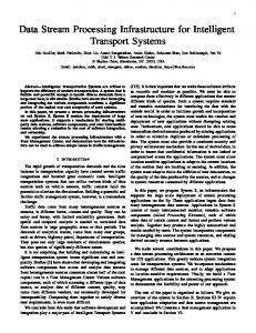
I. I NTRODUCTION Until now, research in the sensor network domain has mainly focused on routing, data aggregation, and energy conservation inside a single sensor network while the intergration of multiple sensor networks has only been studied to a limited extent. However, as the price of wireless sensors diminishes rapidly we can soon expect large numbers of autonomous sensor networks being deployed. These sensor networks will be managed by different organizations but the interconnection of their infrastructures along with data integration and distributed query processing will soon become an issue to fully exploit the potential of this “Sensor Internet.” This requires platforms which enable the dynamic integration and management of sensor networks and the produced data streams. The Global Sensor Networks (GSN) platform aims at providing a flexible middleware to accomplish these goals. GSN assumes the simple model shown in Figure 1: A sensor network internally may use arbitrary multi-hop, ad-hoc routing algorithms to deliver sensor readings to one or more sink node(s). A sink node is a node which is connected to a more powerful base computer which in turn runs the GSN middleware and may particpate in a (large-scale) network of base computers, each running GSN and servicing one or more sensor networks. The work presented in this paper was supported (in part) by the National Competence Center in Research on Mobile Information and Communication Systems (NCCR-MICS), a center supported by the Swiss National Science Foundation under grant no. 5005-67322 and by the L´ıon project supported by Science Foundation Ireland under grant no. SFI/02/CE1/I131.

Fig. 1.

GSN model

We do not make any assumptions on the internals of a sensor network other than that the sink node is connected to the base computer via a software wrapper conforming to the GSN API. On top of this physical access layer GSN provides so-called virtual sensors which abstract from implementation details of access to sensor data and define the data stream processing to be performed. Local and remote virtual sensors, their data streams and the associated query processing can be combined in arbitrary ways and thus enable the user to build a data-oriented “Sensor Internet” consisting of sensor networks connected via GSN. In the follwoing we start with a detailed description of the virtual sensor abstraction in Section II, discuss GSN’s data stream processing and time model in Section III, and present GSN’s system architecture in Section IV. We evaluate the performance of GSN in Section V and discuss related work in Section VI before concluding. II. V IRTUAL

SENSORS

The key abstraction in GSN is the virtual sensor. Virtual sensors abstract from implementation details of access to sensor data and correspond either to a data stream received directly from sensors or to a data stream derived from other virtual sensors. A virtual sensor can be any kind of data producer, for example, a real sensor, a wireless camera, a desktop computer, a cell phone, or any combination of virtual sensors. A virtual sensor may have any number of input data streams and produces exactly one output data stream based on the input data streams and arbitrary local processing. The specification of a virtual sensor provides all necessary information required for deploying and using it, including (1) metadata used for identification and discovery, (2) the structure of the data streams which the virtual sensor consumes and produces (3) an SQL-based specification of the stream processing performed in a virtual sensor, and (4) functional





processing systems. The structure of the data stream a virtual sensor produces is encoded in XML as shown in lines 7– 10. The structure of the input streams is learned from the respective specifications of their virtual sensor definitions. Data stream processing is separated into two stages: (1) processing applied to the input streams (lines 20, 28, and 36) and (2) processing for combining data from the different input streams and producing the output stream (lines 38–43). To specify the processing of the input streams we use SQL queries which refer to the input streams by the reserved keyword WRAPPER. The attribute wrapper="remote" indicates that the data stream is obtained through the network from another GSN instance. In the case of a directly connected local sensor, the wrapper attribute would reference the required wrapper. For example, wrapper="tinyos" would denote a TinyOSbased sensor whose data stream is accessed via GSN’s TinyOS wrapper. GSN already includes wrappers for all major TinyOS platforms (Mica2, Mica2Dot, etc.), for wired and wireless (HTTP-based) cameras (e.g., AXIS 206W), several RFID readers (Texas Instruments, Alien Technology), Bluetooth devices, Shockfish, WiseNodes, epuck robots, etc. The implementation effort for wrappers is rather low, for example, the RFID reader wrapper has 50 lines of code (LOC), the TinyOS 2.x wrapper   has 80 LOC, and the generic serial wrapper has 180 LOC. In the given example the output stream joins the data Fig. 2. A virtual sensor definition received from two temperature sensors and returns a camera image if certain conditions on the temperature are satisfied properties related to persistency, error handling, life-cycle, (lines 38–43). To enable the SQL statement in lines 39–42 to management, and physical deployment. produce the output stream, it needs to be able to reference To support rapid deployment, these properties of virtual the required input data streams which is accomplished by sensors are provided in a declarative deployment descriptor. the alias attribute (lines 14, 22, and 30) that defines a Figure 2 shows an example which defines a virtual sensor that symbolic name for each input stream. The definition of the reads two temperature sensors and in case both of them have structure of the output stream directly relates to the data stream the same reading above a certain threshold in the last minute, processing that is performed by the virtual sensor and needs to the virtual sensor returns the latest picture from the webcam be consistent with it, i.e., the data fields in the select clause in the same room together with the measured temperature. (line 40) must match the definition of the output stream in lines A virtual sensor has a unique name (the name attribute 7–10. in line 1) and can be equipped with a set of key-value In the design of GSN specifications we decided to separate pairs (lines 2–5), i.e., associated with metadata. Both types the temporal aspects from the relational data processing using of addressing information can be registered and discovered SQL. The temporal processing is controlled by various atin GSN and other virtual sensors can use either the unique tributes provided in the input and output stream specifications, name or logical addressing based on the metadata to refer to e.g., the attribute storage-size (lines 14, 22, and 30) a virtual sensor. The example specification above defines a defines the time window used for producing the input stream’s virtual sensor with three input streams which are identified data elements. Due to its specific importance the temporal by their metadata (lines 17–18, 25–26, and 33–34), i.e., by processing will be discussed in detail in Section III. logical addressing. For example, the first temperature sensor In addition to the specification of the data-related propis addressed by specifying two requirements on its metadata erties a virtual sensor also includes high-level specifica(lines 25–26), namely that it is of type temperature sensor and tions of functional properties: The priority attribute (line at a certain physical certain location. By using multiple input 1) controls the processing priority of a virtual sensor, the streams Figure 2 also demonstrates GSN’s ability to access element (line 6) enables the control and multiple stream producers simultaneously. For the moment, management of resources provided to a virtual sensor such we assume that the input streams (two temperature sensors and as the maximum number of threads/queues available for proa webcam) have already been defined in other virtual sensor cessing, the element (line 11) allows the user definitions (how this is done, will be described below). to control how output stream data is persistently stored, and In GSN data streams are temporal sequences of timestamped the disconnect-buffer-size attribute (lines 15, 23, tuples. This is in line with the model used in most stream 31) specifies the amount of storage provided to deal with 1 2 3 BC143 4 room monitoring 5 6 7 8 9 10 11 12 13 14 16 17 BC143 18 Camera 19 20 select * from WRAPPER 21 22 24 25 temperature 26 BC143-N 27 28 select AVG(temp1) as T1 from WRAPPER 29 30 32 33 temperature 34 BC143-S 35 36 select AVG(temp2) as T2 from WRAPPER 37 38 39 select cam.picture as image, temperature.T1 as temp 40 from cam, temperature1 41 where temperature1.T1 > 30 AND 42 temperature1.T1 = temperature2.T2 43 44 45 46

temporary disconnections. For example, in Figure 2 the priority attribute in line 1 assigns a priority of 11 to this virtual sensor (10 is the lowest priority and 20 the highest, default is 10), the element in line 6 specifies a maximum number of 10 threads, which means that if the pool size is reached, data will be dropped (if no pool size is specified, it will be controlled by GSN depending on the current load), the element in line 11 defines that the output stream’s data elements of the last 10 hours (history-size attribute) are stored permanently to enable off-line processing, the storage-size attribute in line 14 defines that the last image taken by the webcam will be returned irrespective of the time it was taken, whereas the storage-size attributes in lines 22 and 30 define a time window of one minute for the amount of sensor readings subsequent queries will be run on, i.e., the AVG operations in lines 28 and 36 are executed on the sensor readings received in the last minute which of course depends on the rate at which the underlying temperature virtual sensor produces its readings, and finally, the disconnect-buffer-size attributes in lines 15, 23, and 31 specify up to 10 missed sensor readings to be read after a disconnection from the associated stream source. The query producing the output stream (lines 39–42) also demonstrates another interesting capability of GSN as it also mediates among three different flavors of queries: The virtual sensor itself uses continuous queries on the temperature data, a “normal” database query on the camera data and produces a result only if certain conditions are satisfied, i.e., a notification analogous to pub/sub or active rules. Virtual sensors are a powerful abstraction mechanism which enables the user to declaratively specify sensors and combinations of arbitrary complexity. Virtual sensors can be defined and deployed to a running GSN instance at any time without having to stop the system. Also dynamic unloading is supported but should be used carefully as unloading a virtual sensor may have undesired (cascading) effects. Due to space limitations we cannot describe all possible configuration options, for example, how virtual sensors are mapped to wrappers which facilitate the physical access or the various notification possibilities, such as email or SMS. A complete list along with a user manual and examples is available from the GSN website at http://gsn.sourceforge.net/. III. DATA STREAM

PROCESSING AND TIME MODEL

Data stream processing has received substantial attention in the recent years in other application domains, such as network monitoring or telecommunications. As a result, a rich set of query languages and query processing approaches for data streams exist on which we can build. A central building block in data stream processing is the time model as it defines the temporal semantics of data and thus determines the design and implementation of a system. Currently, most stream processing systems use a global reference time as the basis for their temporal semantics because they were designed for centralized architectures in the first place. As GSN is targeted at enabling

a distributed “Sensor Internet,” imposing a specific temporal semantics seems inadequate and maintaining it might come at unacceptable cost. GSN provides the essential building blocks for dealing with time, but leaves temporal semantics largely to applications allowing them to express and satisfy their specific, largely varying requirements. In our opinion, this pragmatic approach is viable as it reflects the requirements and capabilities of sensor network processing. In GSN a data stream is a set of timestamped tuples. The order of the data stream is derived from the ordering of the timestamps and GSN provides basic support for managing and manipulating the timestamps. The following essential services are provided: 1) a local clock at each GSN container; 2) implicit management of a timestamp attribute (TIMEID); 3) implicit timestamping of tuples upon arrival at the GSN container (reception time); 4) a windowing mechanism which allows the user to define count- or time-based windows on data streams. In this way it is always possible to trace the temporal history of data stream elements throughout the processing history. Multiple time attributes can be associated with data streams and can be manipulated through SQL queries. Thus sensor networks can be used as observation tools for the physical world, in which network and processing delays are inherent properties of the observation process which cannot be made transparent by abstraction. Let us illustrate this by a simple example: Assume a bank is being robbed and images of the crime scene taken by the security cameras are transmitted to the police. For the insurance company the time at which the images are taken in the bank will be relevant when processing a claim, whereas for the police report the time the images arrived at the police station will be relevant to justify the time of intervention. Depending on the context the robbery is thus taking place at different times. The temporal processing in GSN is defined as follows: The production of a new output stream element of a virtual sensor is always triggered by the arrival of a data stream element from one of its input streams. Thus processing is event-driven and the following processing steps are performed: 1) By default the new data stream element is timestamped using the local clock of the virtual sensor provided that the stream element had no timestamp. 2) Based on the timestamps for each input stream the stream elements are selected according to the definition of the time window and the resulting sets of relations are unnested into flat relations. 3) The input stream queries are evaluated and stored into temporary relations. 4) The output query for producing the output stream element is executed based on the temporary relations. 5) The result is permanently stored if required (possibly after some processing) and all consumers of the virtual sensor are notified of the new stream element.

Stream elements coming from stream source

Stream data element

Stream elements coming from stream source

Stream data element

Timestamp

Timestamp

Persistent storage

Stream Source Query1

Stream Source Query2

Output Relation

Output Relation ...

... Input Stream Query Set of stream elements

Virtual Sensor’s Main Java Class

Fig. 3.

Conceptual data flow in a GSN node

Figure 3 shows the logical data flow inside a GSN node. Additionally, GSN provides a number of possibilities to control the temporal processing of data streams, e.g.: • The rate of a data stream can be bounded in order to avoid overloading the system which might cause undesirable delays. • Data streams can be sampled to reduce the data rate. • A windowing mechanism can be used to limit the amount of data that needs to be stored for query processing. Windows can be defined using absolute, landmark, or sliding intervals. • The lifetime of data streams and queries can be bounded such that they only consume resources when actually active. Lifetimes can be specified in terms of explicit start and end times, start time and duration, or number of tuples. As tuples (sensor readings) are timestamped, queries can also deal explicitly with time. For example, the query in lines 39–42 of Figure 2 could be extended such that it explicitly specifies the maximum time interval between the readings of the two temperatures and the maximum age of the readings. This would additionally require changes in the input stream definitions as the input streams then must provide this information, and also the averaging of the temperature readings (lines 28 and 36) would have to be changed to be explicit in respect to the time dimension. Additionally, GSN supports the integration of continuous and historical data. For example, if the user wants to be notified when the temperature is 10 degrees above the average temperature in the last 24 hours, he/she can simply define two stream sources, getting data from the same wrapper but with different window sizes, i.e., 1 (count) and 24h (time), and then simply write a query specifying the original condition with these input streams. To specify the data stream processing a suitable language is needed. A number of proposals exist already, so we compare the language approach of GSN to the major proposals from the literature. In the Aurora project [5] (http://www.cs.brown.edu/

research/aurora/) users can compose stream relationships and construct queries in a graphical representation which is then used as input for the query planner. The Continuous Query Language (CQL) suggested by the STREAM project [2] (http: //www-db.stanford.edu/stream/) extends standard SQL syntax with new constructs for temporal semantics and defines a mapping between streams and relations. Similarly, in Cougar [13] (http://www.cs.cornell.edu/database/cougar/) an extended version of SQL is used, modeling temporal characteristics in the language itself. The StreaQuel language suggested by the TelegraphCQ project [3] (http://telegraph.cs.berkeley.edu/) follows a different path and tries to isolate temporal semantics from the query language through external definitions in a Clike syntax. For example, for specifying a sliding window for a query a for-loop is used. The actual query is then formulated in an SQL-like syntax. GSN’s approach is related to TelegraphCQ’s as it separates the time-related constructs from the actual query. Temporal specifications, e.g., the window size and rates, are specified in XML in the virtual sensor specification, while data processing is specified in SQL. At the moment GSN supports SQL queries with the full range of operations allowed by the standard SQL syntax, i.e., joins, subqueries, ordering, grouping, unions, intersections, etc. The advantage of using SQL is that it is wellknown and SQL query optimization and planning techniques can be directly applied. IV. S YSTEM

ARCHITECTURE

GSN uses a container-based architecture for hosting virtual sensors. Similar to application servers, GSN provides an environment in which sensor networks can easily and flexibly be specified and deployed by hiding most of the system complexity in the GSN container. Using the declarative specifications, virtual sensors can be deployed and reconfigured in GSN containers at runtime. Communication and processing among different GSN containers is performed in a peer-to-peer style through standard Internet and Web protocols. By viewing GSN containers as cooperating peers in a decentralized system, we tried avoid some of the intrinsic scalability problems of many other systems which rely on a centralized or hierarchical architecture. Targeting a “Sensor Internet” as the long-term goal we also need to take into account that such a system will consist of “Autonomous Sensor Systems” with a large degree of freedom and only limited possibilities of control, similarly as in the Internet. Figure 4 shows the layered architecture of a GSN container. Each GSN container hosts a number of virtual sensors it is responsible for. The virtual sensor manager (VSM) is responsible for providing access to the virtual sensors, managing the delivery of sensor data, and providing the necessary administrative infrastructure. The VSM has two subcomponents: The life-cycle manager (LCM) provides and manages the resources provided to a virtual sensor and manages the interactions with a virtual sensor (sensor readings, etc.). The input stream manager (ISM) is responsible for managing the streams, allocating resources to them, and enabling resource

Integrity service Access control

Query Manager

GSN/Web/Web−Services Interfaces Notification Manager Query Processor Query Repository Storage Virtual Sensor Manager Life Cycle

Input Stream Manager

Manager

Stream Quality Manager

Pool of Virtual Sensors

Fig. 4.

GSN container architecture

sharing among them while its stream quality manager subcomponent (SQM) handles sensor disconnections, missing values, unexpected delays, etc., thus ensuring the QoS of streams. All data from/to the VSM passes through the storage layer which is in charge of providing and managing persistent storage for data streams. Query processing in turn relies on all of the above layers and is done by the query manager (QM) which includes the query processor being in charge of SQL parsing, query planning, and execution of queries. The query repository manages all registered queries (subscriptions) and defines and maintains the set of currently active queries for the query processor. The notification manager deals with the delivery of events and query results to registered, local or remote consumers. The notification manager has an extensible architecture which allows the user to largely customize its functionality, for example, having results mailed or being notified via SMS. The top three layers of the architecture deal with access to the GSN container. The interface layer provides access functions for other GSN containers and via the Web (through a browser or via web services). These functionalities are protected and shielded by the access control layer providing access only to entitled parties and the data integrity layer which provides data integrity and confidentiality through electronic signatures and encryption. Data access and data integrity can be defined at different levels, for example, for the whole GSN container or at a virtual sensor level. An interesting feature of GSN’s architecture is the support for sensor mobility based on automatic detection of sensors and zero-programing deployment: A large number of sensors already support the IEEE 1451 standard which describes a

sensor’s properties and measurement characteristics such as type of measurement, scaling, and calibration information in a so-called Transducer Electronic Data Sheet (TEDS) which is stored inside the sensor. When a new sensor node is detected by GSN, for example, by moving into the transmission range of a sink node, GSN requests its TEDS and uses the contained information for the dynamic generation of a virtual sensor description by using a virtual sensor description template and deriving the sensor-specific fields of the template from the data extracted from the TEDS. At the moment TEDS provides only that information about a sensor which enables interaction with it. Thus for some parts of the generated virtual sensor description, e.g., security requirements, storage and resource management, etc., we use default values. Then GSN dynamically instantiates the new virtual sensor based on this synthesized description and all local and remote processing dependent on the new sensor is executed. This is done on-thefly while GSN is running. The inverse process is performed if a sensor is no longer associated with a GSN node, e.g., it has moved away. In connection with RFID tags this “plug-and-play” feature of GSN even provides new and interesting types of mobility which we will investigate in future work. For example, an RFID tag may store queries which are executed as soon as the tag is detected by a reader, thus transforming RFID tags from simple means for identification and description into a container for physically mobile queries which opens up new and interesting possibilities for mobile information systems. V. E VALUATION GSN aims at providing a zero-programming and efficient infrastructure for large-scale interconnected sensor networks. To justify this claim we experimentally evaluate the throughput of the local sensor data processing and the performance and scalability of query processing as the key influencing factors. As virtual sensors are addressed explicitly and GSN nodes communicate directly in a point-to-point (peer-to-peer) style, we can reasonably extrapolate the experimental results presented in this section to larger network sizes. For our experiments, we used the setup shown in Figure 5. The GSN network consisted of 5 standard Dell desktop PCs with Pentium 4, 3.2GHz Intel processors with 1MB cache, 1GB memory, 100Mbit Ethernet, running Debian 3.1 Linux with an unmodified kernel 2.4.27. For the storage layer use standard MySQL 5.18. The PCs were attached to the following sensor networks as shown in Figure 5. • A sensor network consisting of 10 Mica2 motes, each mote being equipped with light and temperature sensors. The packet size was configured to 15 Bytes (data portion excluding the headers). • A sensor network consisting of 8 Mica2 motes, each equipped with light, temperature, acceleration, and sound sensors. The packet size was configured to 100 Bytes (data portion excluding the headers). The maximum possible packet size for TinyOS 1.x packets of the current TinyOS implementation is 128 bytes (including headers).

30 15 bytes 50 bytes 100 bytes 16KB 32KB 75 KB

Processing Time in (ms)

25

20

15

10

5

0 0

100

200

Fig. 6. Tinynode

TI-RFID Reader/Writer

Fig. 5.

AXIS 206W

Mica2 with housing box

300

400 500 600 Output Interval (ms)

700

800

900

1000

GSN node under time-triggered load

WRT54G

Experimental setup

A sensor network consisting of 4 Tiny-Nodes (TinyOS compatible motes produced by Shockfish, http://www. shockfish.com/), each equipped with a light and two temperature sensors with TinyOS standard packet size of 29 Bytes. • 15 Wireless network cameras (AXIS 206W) which can capture 640x480 JPEG pictures with a rate of 30 frames per second. 5 cameras use the highest available compression (16kB average image size), 5 use medium compression (32kB average image size), and 5 use no compression (75kB average image size). The cameras are connected to a Linksys WRT54G wireless access point via 802.11b and the access point is connected via 100Mbit Ethernet to a GSN node. • A Texas Instruments Series 6000 S6700 multi-protocol RFID reader with three different kind of tags, which can keep up to 8KB of data. 128 Bytes capacity. The motes in each sensor network form a sensor network and routing among the motes is done with the surge multi-hop ad-hoc routing algorithm provided by TinyOS. •

A. Internal processing time In the first experiment we wanted to determine the internal processing time a GSN node requires for processing sensor readings, i.e., the time interval when the wrapper gets the sensor data until the data can be provided to clients by the associated virtual sensor. This delay depends on the size of the sensor data and the rate at which the data is produced, but is independent of the number of clients wanting to receive the sensor data. Thus it is a lower bound and characterizes the efficiency of the implementation. We configured the 22 motes and 15 cameras to produce data every 10, 25, 50, 100, 250, 500, and 1000 milliseconds. As the cameras have a maximum rate of 30 frames/second, i.e., a frame every 33 milliseconds, we added a proxy between

the GSN node and the WRT54G access point which repeated the last available frame in order to reach a frame interval of 10 milliseconds. All GSN instances used the Sun Java Virtual Machine (1.5.0 update 6) with memory restricted to 64MB. The experiment was conducted as follows: All motes and cameras were set to the same rate and produced data for 8 hours and we measured the processing delay. This was repeated 3 times for each rate and the measurements were averaged. Figure 6 shows the results of the experiment for the different data sizes produced by the motes and the cameras. High data rates put some stress on the system but the absolute delays are still quite tolerable. The delays drop sharply if the interval is increased and then converge to a nearly constant time at a rate of approximately 4 readings/second or less. This result shows that GSN can tolerate high rates and incurs low overhead for realistic rates as in practical sensor deployments lower rates are more probable due to energy constraints of the sensor devices while still being able to deal also with high rates. B. Scalability in the number of queries and clients In this experiment the goal was to measure GSN’s scalability in the number of clients and queries. To do so, we used two 1.8 GHz Centrino laptops with 1GB memory as shown in Figure 5 which each ran 250 lightweight GSN instances. The lightweight GSN instance only included those components that we needed for the experiment. Each GSN-light instance used a random query generator to generate queries with varying table names, varying filtering condition complexity, and varying configuration parameters such as history size, sampling rate, etc. For the experiments we configured the query generator to produce random queries with 3 filtering predicates in the where clause on average, using random history sizes from 1 second up to 30 minutes and uniformly distributed random sampling rates (seconds) in the interval [0.01, 1]. Then we configured the motes such that they produce a measurement each second but would deliver it with a probability P < 1, i.e., a reading would be dropped with probability 1 − P > 0. Additionally, each mote could produce

50

SES=30Bytes

SES = 100 Bytes SES = 15 KB SES = 25 KB

40

Avg Processing Time for each client (ms)

Total processing time (ms) for the set of clients

12

30

20

10

10

8

6

4

2

0

0 0

100

Fig. 7.

200 300 Number of Clients

400

500

Query processing latencies in a node

a burst of R readings at the highest possible speed depending on the hardware with probability B > 0, where R is a uniformly random integer from the interval [1, 100]. I.e., a burst would occur with a probability of P ∗ B and would produce randomly 1 up to 100 data items. In the experiments we used P = 0.85 and B = 0.3. On the desktops we used MySQL as the database with the recommended configuration for large memory systems. Figure 7 shows the results for a stream element size (SES) of 30 Bytes. Using SES=32KB gives the same latencies. Due to space limitations we do not include this figure. The spikes in the graphs are bursts as described above. Basically this experiment measures the performance of the database server under various loads which heavily depends on the used database. As expected the database server’s performance is directly related to the number of the clients as with the increasing number of clients more queries are sent to the database and also the cost of the query compiling increases. Nevertheless, the query processing time is reasonably low as the graphs show that the average time to process a query if 500 clients issue queries is less than 50ms, i.e., approximately 0.5ms per client. If required, a cluster could be used to the improve query processing times which is supported by most of the existing databases already. In the next experiment shown in Figure 8 we look at the average processing time for a client excluding the query processing part. In this experiment we used P = 0.85, B = 0.05, and R is as above. We can make three interesting observations from Figure 8: 1) GSN only allocates resources for virtual sensors that are being used. The left side of the graph shows the situation when the first clients arrive and use virtual sensors. The system has to instantiate the virtual sensor and activates the necessary resources for query processing, notification, connection caching, etc. Thus for the first clients to arrive average processing times are a bit higher. CPU usage is around 34% in this interval. After a short time (around 30 clients) the initialization phase is over

0

100

200 300 Number of clients

Fig. 8.

400

500

Processing time per client

and the average processing time decreases as the newly arriving clients can already use the services in place. CPU usage then drops to around 12%. 2) Again the spikes in the graph relate to bursts. Although the processing time increases considerably during the bursts, the system immediately restores its normal behavior with low processing times when the bursts are over, i.e., it is very responsive and quickly adopts to varying loads. 3) As the number of clients increases, the average processing time for each client decreases. This is due to the implemented data sharing functionalities. As the number of clients increases, also the probability of using common resources and data items grows. VI. R ELATED WORK So far only few architectures to support interconnected sensor networks exist. Sgroi et al. [11] suggest basic abstractions, a standard set of services, and an API to free application developers from the details of the underlying sensor networks. However, the focus is on systematic definition and classification of abstractions and services, while GSN takes a more general view and provides not only APIs but a complete query processing and management infrastructure with a declarative language interface. Hourglass [12] provides an Internet-based infrastructure for connecting sensor networks to applications and offers topicbased discovery and data-processing services. Similar to GSN it tries to hide internals of sensors from the user but focuses on maintaining quality of service of data streams in the presence of disconnections while GSN is more targeted at flexible configurations, general abstractions, and distributed query support. HiFi [7] provides efficient, hierarchical data stream query processing to acquire, filter, and aggregate data from multiple devices in a static environment while GSN takes a peer-to-peer perspective assuming a dynamic environment and allowing any node to be a data source, data sink, or data aggregator.

IrisNet [8] proposes a two-tier architecture consisting of sensing agents (SA) which collect and pre-process sensor data and organizing agents (OA) which store sensor data in a hierarchical, distributed XML database. This database is modeled after the design of the Internet DNS and supports XPath queries. X-Tree [] extends IrisNet by providing a database centric programming model (stored functions and stored queries) with efficient distributed execution. In contrast to that, GSN follows a symmetric peer-to-peer approach as already mentioned and supports relational queries using SQL. Rooney et al. [10] propose so-called EdgeServers to integrate sensor networks into enterprise networks. EdgeServers filter and aggregate raw sensor data (using application specific code) to reduce the amount of data forwarded to application servers. The system uses publish/subscribe style communication and also includes specialized protocols for the integration of sensor networks. While GSN provides a general-purpose infrastructure for sensor network deployment and distributed query processing, the EdgeServer system targets enterprise networks with application-based customization to reduce sensor data traffic in closed environments. Besides these architectures, a large number of systems for query processing in sensor networks exist. Aurora [5] (Brandeis University, Braun University, MIT), STREAM [2] (Stanford), TelegraphCQ [3] (UC Berkeley), and Cougar [13] (Cornell) have already been discussed and related to GSN in Section III. In the Medusa distributed stream-processing system [14], Aurora is being used as the processing engine on each of the participating nodes. Medusa takes Aurora queries and distributes them across multiple nodes and particularly focuses on load management using economic principles and high availability issues. The Borealis stream processing engine [1] is based on the work in Medusa and Aurora and supports dynamic query modification, dynamic revision of query results, and flexible optimization. These systems focus on (distributed) query processing only, which is only one specific component of GSN, and focus on sensor heavy and server heavy application domains. Additionally, several systems providing publish/subscribestyle query processing comparable to GSN exist, for example, [9]. GSN can also integrate easily existing approaches (as a new virtual sensor) for precision estimation, for example, [6] or aggregation handling uncertainty, for example, [4]. VII. C ONCLUSIONS The full potential of sensor technology will be unleashed through large-scale (up to global scale) data-oriented integration of sensor networks. To realize this vision of a “Sensor Internet” we suggest our Global Sensor Networks (GSN) middleware which enables fast and flexible deployment and interconnection of sensor networks. Through its virtual sensor abstraction which can abstract from arbitrary stream data sources and its powerful declarative specification and query tools, GSN provides simple and uniform access to the host of heterogeneous technologies. GSN offers zero-programming

deployment and data-oriented integration of sensor networks and supports dynamic configuration and adaptation at runtime. Zero-programming deployment in conjunction with GSN’s plug-and-play detection and deployment feature provides a basic functionality to enable sensor mobility. GSN is implemented in Java and C/C++ and is available from SourceForge at http://gsn.sourcefourge.net/. The experimental evaluation of GSN demonstrates that the implementation is highly efficient, offers very good performance and throughput even under high loads and scales gracefully in the number of nodes, queries, and query complexity. R EFERENCES [1] Daniel J. Abadi, Yanif Ahmad, Magdalena Balazinska, Ugur C ¸ etintemel, Mitch Cherniack, Jeong-Hyon Hwang, Wolfgang Lindner, Anurag Maskey, Alex Rasin, Esther Ryvkina, Nesime Tatbul, Ying Xing, and Stanley B. Zdonik. The Design of the Borealis Stream Processing Engine. In CIDR, 2005. [2] A. Arasu, B. Babcock, S. Babu, J. Cieslewicz, M. Datar, K. Ito, R. Motwani, U. Srivastava, and J. Widom. Data-Stream Management: Processing High-Speed Data Streams, chapter STREAM: The Stanford Data Stream Management System. Springer, 2006. [3] Sirish Chandrasekaran, Owen Cooper, Amol Deshpande, Michael J. Franklin, Joseph M. Hellerstein, Wei Hong, Sailesh Krishnamurthy, Samuel Madden, Vijayshankar Raman, Frederick Reiss, and Mehul A. Shah. TelegraphCQ: Continuous Dataflow Processing for an Uncertain World. In CIDR, 2003. [4] Reynold Cheng, Dmitri V. Kalashnikov, and Sunil Prabhakar. Evaluating Probabilistic Queries over Imprecise Data. In SIGMOD, 2003. [5] Mitch Cherniack, Hari Balakrishnan, Magdalena Balazinska, Donald Carney, Ugur C ¸ etintemel, Ying Xing, and Stanley B. Zdonik. Scalable Distributed Stream Processing. In CIDR, 2003. [6] Amol Deshpande and Samuel Madden. MauveDB: Supporting Modelbased User Views in Database Systems. In SIGMOD, 2006. [7] M. Franklin, S. Jeffery, S. Krishnamurthy, F. Reiss, S. Rizvi, E. Wu, O. Cooper, A. Edakkunni, and W. Hong. Design Considerations for High Fan-in Systems: The HiFi Approach. In CIDR, 2005. [8] P. B. Gibbons, B. Karp, Y. Ke, S. Nath, and S. Seshan. IrisNet: An Architecture for a World-Wide Sensor Web. IEEE Pervasive Computing, 2(4), 2003. [9] A. J. G. Gray and W. Nutt. A Data Stream Publish/Subscribe Architecture with Self-adapting Queries. In International Conference on Cooperative Information Systems (CoopIS), 2005. [10] Sean Rooney, Daniel Bauer, and Paolo Scotton. Techniques for Integrating Sensors into the Enterprise Network. IEEE eTransactions on Network and Service Management, 2(1), 2006. [11] M. Sgroi, A. Wolisz, A. Sangiovanni-Vincentelli, and J. M. Rabaey. A service-based universal application interface for ad hoc wireless sensor and actuator networks. In Ambient Intelligence. Springer Verlag, 2005. [12] J. Shneidman, P. Pietzuch, J. Ledlie, M. Roussopoulos, M. Seltzer, and M. Welsh. Hourglass: An Infrastructure for Connecting Sensor Networks and Applications. Technical Report TR-21-04, Harvard University, EECS, 2004. http://www.eecs.harvard.edu/∼ syrah/hourglass/ papers/tr2104.pdf. [13] Yong Yao and Johannes Gehrke. Query Processing in Sensor Networks. In CIDR, 2003. [14] Stan Zdonik, Michael Stonebraker, Mitch Cherniack, Ugur Cetintemel, Magdalena Balazinska, and Hari Balakrishnan. The Aurora and Medusa Projects. Bulletin of the Technical Committe on Data Engineering, IEEE Computer Society, 2003.