W I N D E N G I N E E R I N G V O L U M E 27, N O . 1, 2003
PP
21 38
21
Initialisation of Grid-Connected Wind Turbine Models in Power-System Simulations Anca D. Hansen*, Poul Sørensen*, Florin Iov+ and Frede Blaabjerg+ *Risø National Laboratory, Wind Energy Department, P.O. Box 49, DK-4000 Roskil de, Denmark Email:* <
[email protected]> +Aalborg University, Institute of Energy Technology, Pontoppidanstræde 10 1, DK-9220 Aalborg East, Denmark
ABSTRACT This paper describes a method of initi alisi ng dynamic wi nd turbi ne models in pow er-system simulations. The method uses grid-status information to initi alise the grid-connected wind turbine model. The goal is to start a power-system simulation in a stati onary state, without unnecessary transient behaviour at the beginning of the simulation. Correct initialisati on is necessary to reach quickly the steady state of the grid-connected wi nd turbine, before a real transient on the grid occurs. Consequently, the dynami c performance of the system can be independently and accurately evaluated. The method presented considers wi nd turbines with directl y grid-connected induction generators, wi th constant or variable blade angle (passive stall control, blade angle control or active stall control). These aspects apply to both constant and vari able speed wi nd turbi nes. The investigati on is performed in the commercial dedicated power-system simulation-tool DIgSILENT. Attention is especially drawn to the initi alisation of the non-electrical parts of the wind turbine. The suitability of this initialisation strategy is illustrated by an ex ample. K ey words: model initiali sati on, wind turbine, grid interacti on, pow er system, dynami c simulation, DIgSILENT
1. INTRODUCTION In the last few years, increased and concentrated penetration of wind energy into electrical power-systems has made the latter more vulnerable and dependent on the wind energy production. Moreover, future wind turbines must be able to replace conventional power stations, and thus be active and controllable elements in the power supply network (Sørensen P. et al., 2000). Obviously, interaction of wind turbines with electrical power-systems is becoming more significant. Therefore, it is important to perform new studies of power-system dynamics in order to investigate all the aspects related to the interaction between wind turbines and the power-system both during normal operation and during transient gri d faults. Also, proper integration of wind turbine models within power-system simulation is of great importance for the analysis of wind energy penetration and power-system performance. Indeed, actual integration of large wind farms with the grid may use similar methods. The integration of the models into the pow er system si mulation requires proper initialisation of the dynamic wind turbine models based on the steady state load flow data of the electrical power system at the point of connection. Correct initialisation avoids false electrical transients (due to wrong initialisation). The dynamic performance of the gri dconnected wind turbine, even in the case of a grid transient event, can be thus evaluated
22
I N I T I A L I S AT I O N
OF
G R I D- C O N N E C T E D W I N D T U R B I N E M O D E L S
IN
P OW E R - S Y S T E M S I M U L AT I O N S
accurately. This initialisation requires the wind turbine and the electrical power-system to be treated as a unified/whole system, despite their formal separation at initialisation. The proposed method calculates the initial conditions of the dynamic wind turbine models, based partially on power-system load flow data and on a prior knowledge of the wind speed and blade angle of the wind turbine. This implies that the initialisation sequence is based on both (i) information from the grid to the wind turbine, and (ii) information from the wind turbine to the grid. Notice that the direction of initialisation from grid to the wind turbine is not a conventional direction, being opposite to the direction of the simulation. The paper presents some results of a national Danish research project (Aalborg Universi ty & Ri sø, 2002), whose overall objective is to create a model database in different simulation tools, able to support the analysis of the interaction between the mechanical structure of the wind turbine and the electrical grid during different operational modes. Such developed models enable both the wind turbine investors and the grid utility technical staff to perform the necessary preliminary studies before investing and connecting wind turbines (farms) to the grid. Simulation of the wind turbine interaction with the grid may thus provide valuable information and may even lower overall grid connection costs. In this paper, the attention is mainly drawn to the initialisation of the models of the nonelectrical wind turbine components. The initialisation of the electrical machine models is, in the present work, performed by the si mulation-tool DIgSILENT. It is beyond the scope of this paper, being described in several references e.g. (Slootweg et al., 2001), (Akhmatov, 2002). This paper focuses on the initialisation of a blade-angle controlled wind turbine, with a directl y gri d-connected squirrel -cage induction generator. The wind turbine model, implemented in the commercially available software tool DIgSILENT for power-system simulation, comprises (a) the station where the wind turbine is connected, (b) the powe r collection system (transformers, cables, busbar), (c) the electric, mechanical, aerodynami c models of the wind turbine and the wind model. The purpose of the model is to enable assessment of power quality, control strategies and behaviour of the wind turbine in the event of grid faults.
2. GRID-CONNECTED WIND TURBINE MODEL AND INITIALISATION STRATEGY 2.1. Power-System Simulation-Tool: DIgSILENT The increasing capacity of wind penetration is one of today’s most challenging aspects in power-system control. Computer models of power systems are widely used by power-system utilities to study load flow, steady state voltage stability, dynamic and transient behaviour of power systems. Today these tools must incorporate extensive modelling capabilities with a d vanced solution algorithms for complex power-system studies, as in the case of wind powe r applications. An example of such a tool is the dedicated power-system si mulation-tool DIgSILENT (DIgSILENT GmbH, 2003). DIgSILENT has the ability to simulate load flow, RMS fluctuations and transient events in the same software environment. It provides models with different detailing in a structured w ay. It combines models for electromagnetic transient simulations of instantaneous values with models for electromechanical si mulations of RMS values. This makes the models useful for studies of both (transient) grid fault and (longer-term) power quality and control issues. DIgSILENT provides a comprehensive library of models for electrical components in power systems. Models include e.g. generators, motors, controllers, dynamic loads and various passive network elements (e.g. lines, transformers, static loads and shunts). Therefore, in the present work, the grid model and the electrical components of the wind turbine model are
W I N D E N G I N E E R I N G V O L U M E 27, N O . 1, 2003
23
included as standard components in the existing library. Similarl y, the models of the wind speed, of the mechanical, aerodynamic and control systems of the wind turbines are written in the dynamic si mulation language DSL of DIgSILENT, which makes it possible for users to create their own blocks either as modifications of existing models or as completely new models. These new models can be gathered in a library, which can be easily used further in the modelling of other wind farms with other wind turbines.
2.2. Grid-Connected Wind Turbine Model This paper emphasises the initialisation aspects of the models of the non-electrical wind turbine components. It is therefore beyond the scope of this paper to present a detailed description of the model of the grid-connected wind turbine and of the wind speed, as more details can be found in (Sørensen P. et al., 2001a) and (Sørensen P. et al., 2001b). The grid-connected wind turbine model implemented in DIgSILENT includes a grid model and a wind turbine model. In this paper, a typical blade angle controlled wind turbine with a squirrel-cage induction generator, connected directly to the grid, is considered. The wind turbine’s rotor is coupled to the generator through a gearbox, the power extracted from the wind is limited using blade angle control and the compensation for the consumed reactive power in the magnetisation of the induction generator is done with the help of a capacitor bank.
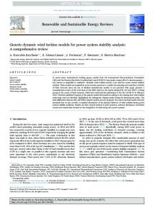
(a) Grid model An ex ample of a grid model is depicted in Figure 1. It contains the connection of the wind turbine to the station and the electrical part of the wind turbine from the tower bottom to the nacelle at the tower top. The connection of the wind turbine to the station is modelled by the actual physical component models from DIgSILENT library (transformer, line, load, busbar), while the remai ning power-system is represented by si mplified equivalents, as e.g. a Thevenin equivalent models the grid. This is a reasonable approximation for power quality studies, as the grid is assumed very strong as compared to the power capacity of the wind turbine. Grid Thevenin equivalent V ~
Station
Load Transformer Capacitor bank Main switch point (MSP)
Terminal bottom
C
Tower cable
C
Terminal nacelle
G ~
Figure 1.
E xample of the configuration of a grid model and an electrical model of the wind turbine with a squirrel cage generator.
The electrical model of the turbine includes DIgSILENT models for the induction generator and the capacitor bank for reactive power compensation. The capacitor bank, with a specific number of capacitors, is controlled by information of the measured reactive power Q meas (a t
24
I N I T I A L I S AT I O N
OF
G R I D- C O N N E C T E D W I N D T U R B I N E M O D E L S
IN
P OW E R - S Y S T E M S I M U L AT I O N S
the Main Switch Point of the wind turbine) and on the operational status of each capacitor d c, namely information on how many capacitors are open/closed at a certain instant. The electrical control system model, implemented in the dynamic si mulation language (DSL), sends the switch signals Sc to the grid model and further to the capacitor bank contacts, in order to connect or disconnect the individual capacitors.
(b) Wind turbine model Figure 2 illustrates the overall structure of the grid-connected wind turbine model and the direction of the simulation flow (indicated by solid lines), with the inputs (on left side) and outputs (on right side) of each block model. It contains: (i) the wind speed model, (ii) the aerodynamic, mechanical, electrical models, and (iii) the control system model itself. The wind model generates the equivalent wind speed (eq based on a spectral description of the turbulence and includes the rotational sampling turbulence and of the tower shadow into account (Sørensen P. et al., 2001b). The aerodynamic model contains two sub-models: one 1 expresses the non-linear expression of the aerodynamic torque T = ____ , l ), r p R 2 v3 C ( u 2v
r ot
r ot
eq
p
pi tch
while the other describes the dynamic stall effects (Sørensen P. et al., 2001a). This means that a dynamic aerodynamic efficiency C pdynami c ( u aerodynamic coefficient C p ( u
pitch , l
pi tch,
). The aerodynamic model is fed with the equivalent wind-
speed veq from the wind model, the rotor speed v angle u
pi tch from
l ) is used instead of the steady state
rot
from the mechanical model and the blade
the control model. The mechanical model describes the dynamics of the drive
train and delivers the mechanical turbine power P t to the generator model. Beside the mechanical turbine power P t , the generator model has as input the voltage U gen from the grid model. It delivers the rotational speed v
Blade angle control model q
gen
and the current I gen as outputs.
pitch
Aerodynamic model
n
Dynamic stall effects
eq
n
eq
n
Wind model
eq
C dyn p
Ugen l
Aerodyn. torque
Trot
Pt
Mechanical model
Ugen Generator model
Igen Sc
Grid model
dc Q meas
Capacitor bank control model
P meas MSP
w w q w
rot
w
rot
q
rot
Sc
gen
rot
w
gen
gen
P meas
Figure 2.
Simulation flow in the grid-connected wind turbine model.
The blade angle-control and capacitor-bank electrical control systems constitute the overall control. The blade angle-control model delivers the blade angle u
pi t ch
to the
aerodynamic model, by using information on the measured active power P meas , the generator
W I N D E N G I N E E R I N G V O L U M E 27, N O . 1, 2003
speed v
gen
25
and the wind speed veq. The capacitor-bank control model generates the capacitor
switch control signals SC to the grid model, based on information on the measured reactive power Q meas and on the capacitor status signals d c. The active and the reactive power P meas and Q meas are measured at the main switch point MSP; see Figure 1. The measurements from this point are used by the control system.
2.3. Initialisation Procedure To integrate new models in the power-system simulation software, e.g. for wind turbines and new controllers, the initialisation problem must to be solved properl y. Correct initialisation of a model in a power-system simulation-tool avoids fictitious electrical transients and makes possible to evaluate correctly the real dynamic performance of the system, even in the case of a grid transient event. Simulation by a power-system package, as e.g. DIgSILENT, starts by preparing and solving a load flow case, by using the load-flow calculation module of the software. Load flow input data, representing the operational steady state of the system at the moment of simulation start, are required by the simulation package at the beginning of the simulation. The load flow input data for a squirrel-cage induction generator includes the active power. For a doubly-fed induction generator, the required load flow data are the active power, reactive power and the slip. Once the load flow calculation is accomplished, and thus all electrical models (machines, loads etc) are initialised (e.g. calculating mechanical turbine power at the machine, generator speed at the start moment), the initialisation of the models of the turbine component starts. The electrical data available from the load flow and the equations of grid components are expressed in per unit in DIgSILENT and therefore, as the turbine equations are implemented in physical units, some transformations must be considered in the initialisation of the turbine model. This paper presents an initialisation procedure exemplified for a blade angle controlled wind turbine with a directly connected squirrel -cage induction generator. Howeve r, during the description of this initialisation procedure, some comments regarding the vari able speed wind turbine are also made. The initialisation of the grid-connected turbine model is a successive process. The main issue is to find the sequence in which the models have to be initialised one by one, based on the accomplished data provided by the load flow calculation, on eventual additional nonelectrical input data and on the simulation equations. It is necessary to identify which inputs/outputs/states are known and which have to be initialised. Once one model is initialised, the gathered information on its signals and states is used for the initialisation of the next model. DIgSilent can check if the initial conditions are transferred correctly from one component model to another. If the initialisation is not done properl y, the state variables do not stay at the value at which they were initialised, but start changing at the start of the dynamic simulation. In this case, it may take time to reach a steady state and numerical instability can even occur before the stationary state is reached. These initialisation transients are undesirable in the transient studies of the dynamic performance of the system, especially in the case when a real grid transient event appears just before the system achieves its steady state. A correct evaluation of the dynamic performance is then quite difficult to achieve. Therefore, an accurate calculation of the initial conditions of the dynamic wind turbine models would be extremely helpful. Figure 3 illustrates the initialisation flow of the turbine model and the input data necessary: 1.
electrical input data (from grid side): e.g. the initial active power of the generator
26
I N I T I A L I S AT I O N
OF
G R I D- C O N N E C T E D W I N D T U R B I N E M O D E L S
IN
P OW E R - S Y S T E M S I M U L AT I O N S
and the initial capacitor status information d c . These electrical input data are used in the load flow calculation and in the initialisation of the electrical models. 2.
non-electrical input data (from turbine side): the initial value of the wind speed and the initial value of the blade angle.
These input data provide global information about the operational mode of the turbine at the simulation start. The single-dotted lines indicate the direction of the initialisation flow, for each component model; see Figure 3. The known signals at the simulation start, indicated by the double dotted lines, are: electrical signals determined in the load flow calculation: mechanical power P t ,
1.
generator speed v
gen,
capacitor status signal d c, generator current I gen, generator
voltage U gen, the “measured” active power P meas and reactive power Q meas in MSP (Main Switch Point). a pri ori known non-electrical signals: the initial wind speed veq and the initial blade
2.
angle u
pi tch.
A Initialisation direction from grid side (opposite simulation flow direction)
Initialisation direction from wind turbine side (simulation flow direction)
Initial pitch angle
Blade angle q control model
pitch
Aerodynamic model
n
Dynamic stall effects
Cpdyn
Ugen l
eq
n
Wind model
Initial wind speed
eq
Aerodyn. torque
Trot
Trot
Pt
Mechanical model
Ugen Generator model
Igen Sc
Grid model
dc Qmeas
Capacitor bank control model
Pmeas MSP
w w q w
w
rot
rot
q
rot
Sc
gen
rot
w
gen
gen
Pmeas Initialisation flow
A
Figure 3.
Initialisation flow of the grid-connected wind turbine model.
The non-electrical input data (from the turbine side) and the load flow electrical input data (from the grid side) must correspond to each other, based on the static power curve of the wind turbine and on the generator efficiency. The initial value of the wind speed is assumed known at the beginning of the initialisation sequence because, otherwise, its initialisation
Load flow input data: P gen, d c
W I N D E N G I N E E R I N G V O L U M E 27, N O . 1, 2003
27
b ac k ward from the non-linear expression in wind speed of the aerodynamic torque would be quite difficult and with ambiguous solutions. It is also reasonable to assume a known initial value of the blade angle. There are several reasons: (1)
both pitch control and active stall control turbines can have an optimum aerodynamic coefficient for different values of the blade angle, case that implies multiple possible solutions for the initialisation of the blade angle;
(2 )
in the case of stall controlled wind turbines the blades are pitched to a well know n predefined angle; (3) for variable speed turbines, a pri ori known blade angle u
pitch
makes it possi ble to fully determine/initialise the optimum value of the aerodynamic coefficient C popt for a certain tip speed ratio l . Tw o initialisation directions are distinguished in the initialisation procedure; see Figure 3. Some of the variables in the initialisation sequence are initialised in the opposite direction of the simulation (starting from the grid connection point towards the wind); while others are initialised in the same direction as the simulation is performed (starting from the wind to the grid). When the initialisation is performed in the opposite direction of the simulation flow, namely from the grid to the wind, the model is calculated from certain known output to the input, based on load flow computations. The initial values of the inputs, outputs and state vari ables have thus to be calculated from the known outputs and from the model equations. For example, in the “Mechanical model” block shown in Figure 3, the aerodynamic torque T r ot is initialised in the opposite direction of the simulation flow (illustrated in Figure 2). It is based on the known outputs from the load flow calculation, i.e. the mechanical power P t and the generator speed v
gen.
When the initialisation is performed in the same direction as the
simulation flow, the model is calculated from certain known input to the output. The initial values of the inputs are assumed known based on the non-electrical information about the system in the starting moment, as e.g. the initial wind speed and the initial blade angle. These t wo initialisation directions cross each other at a certain component model. As in this case, the initialisation information is coming from two opposite directions, one should be aware of a possible conflict, which can appear when there is not a full correspondence (concordance) between the load flow input data and the non-electrical input data, namely wind speed and blade angle. This conflict must be avoided. Its effects can be minimised by “placing” the crossing of the initialisation information from opposite directions in that component model, whose si gnals/states can handle eventual conflict steps, by absorbing the transients ve ry quickly. In the present initialisation method, the place between the aerodynamic model and the mechanical model is chosen as the place where the initialisation information is coming from two opposite directions. This is illustrated in Figure 3 by the border line AA«. The reason for this choice is that the transients in the low-speed shaft torque signal, in the case of an initialisation conflict, are absorbed due to the large inertia of the rotor.
3. CALCULATION OF INITIAL CONDITIONS This section explains the calculation of the initial conditions of those turbine component models, which are relevant for a correct initialisation of the whole system (i.e. turbine together with the grid). When the initial conditions are calculated, the system is conditioned to be in steady state (the derivati ves are set to zero). As indicated in Figure 3, the initialisation sequence of the models of the non-electrical turbine components starts with the mechanical model, which receives known signals (on
28
I N I T I A L I S AT I O N
OF
G R I D- C O N N E C T E D W I N D T U R B I N E M O D E L S
IN
P OW E R - S Y S T E M S I M U L AT I O N S
generator and gri d) from the load flow calculation. DIgSILENT automatically performs the initialisation of the generator, in the load-flow calculation step. The models are initialised one by one, starting with the mechanical model, followed by the wind model, blade-angle control-model and the aerodynamic model. The initialisation of the capacitor-bank control model is based on the load flow data only, i.e. independent of the initialisation of the other individual component models. Once one model is initialised, all its variables are known and useable in the initialisation of the next models in the initialisation sequence. In the following figures, related to each component model, the known signals in the initialisation moment are illustrated by using the double-dotted line, while the signals, which must be initialised, are illustrated by single-dotted line.
3.1. Mechanical Model Figure 4 illustrates the inputs and outputs of the mechanical model, which must be initialised. These are the aerodynamic torque T r ot, the rotor angle u mechanical power P tl f and the generator speed v
lf gen
r ot
and the rotor speed v
r ot.
The
are known (double dotted style) from the
load flow calculation. The aerodynamic torque T r ot is initialised in the opposite direction to that of the simulation flow (i.e. from grid to wind, and not from wind to grid), while the rotor angle u
r ot,
the rotor speed v
rot
and the internal states of the mechanical model are initialised in
the same direction as the simulation flow.
T rot w
Figure 4.
lf gen
Pt lf [p.u.]
[Nm] [p. u. ]
Mechanical model
q
w
rot
[rad/s]
rot [rad]
Known and unknown inputs/outputs in the initialisation of the mechanical model.
The per unit mechanical power P tl f and the generator speed v
lf gen,
generated by the load
flow are:
Pt Pt base
Pt lf =
w
lf gen
=
w
w
(1)
gen base gen
where P tbase is the rated mechanical power in [W], v
base gen
= 2__pp__f is the synchronous speed of the
generator in [rad/s], with f as the grid frequency in [Hz] and p as the number of pole-pairs. The mechanical model is essentially a two mass model (Hansen A.D. et al., 2002), (Sørensen P. et al., 2001a), namely a large mass corresponding to the rotor inertia J r ot and a small mass corresponding to the generator inertia J gen, which is implemented as part of a DIgSILENT generator model. Thus, besides the electro-magnetic description, the generator model in DIgSILENT also contains the mechanical inertia of the generator rotor J gen. The low speed shaft is modelled by a stiffness k and a damping coefficient c, while the high-speed shaft is assumed stiff. Moreover, an ideal gear with the ratio (1:ngear) is included. The dri ve train converts the aerodynamic torque T r ot of the rotor into the torque on the low speed shaft T shaft. The dynamical description of the mechanical model consists of three differential equations, namely:
W I N D E N G I N E E R I N G V O L U M E 27, N O . 1, 2003
q ‚rot = w q ‚k = w
29
[rad / s ]
rot
w -
rot
[rad / s ]
gen
n gear
[rad / s ]
w ‚ rot = (Trot - Tshaft ) / J rot where u
k
=u
r ot
u
gen/
(2)
2
n gear is the angular difference between the two ends of the flexible shaft.
The mechanical torque on the low speed shaft and the mechanical power of the generator are:
Tshaft = c (w Pt = w
rot
w -
)+kq
gen
n gear
k
Tshaft gen
[Nm ] (3)
[W ]
ngear
The initial steady states are determined by setting their derivati ves to zero:
q ‚k
= 0
w Þ
w ‚ rot = 0 Þ
initial rot
=
w
gen
n gear
inital inital Trot = Tshaft
and
initial Tshaft =kq
and
Trotinitial =
initial k
(4)
Pt n gear
w
gen
Notice that since the shaft is rotating, the derivati ve of the rotor position u
r ot cannot
be zero.
Its value can be initialised to any appropriate value. The mechanical model, expressed in (2) and (3), is using physical units, while the signals determined in the load flow calculation are expressed in per unit. The initialisation of the inputs and states, based on equations (3) and (4), must take the transformations (1) into account, as follows:
q
T
initial rot
= n gear
w
initial rot
=
initial k
=
w
lf gen
Ptlf Ptbase
w
lf gen
w
w
base gen
base gen
n gear
(5)
P lf P base 1 Trotinitial = n gear tlf t base k w gen w gen k
3.2. Wind Model The result of the wind model is an equivalent wind-speed veq, which is further used as input into the aerodynamic model and in the blade-angle control block; see Figure 2. The initial value of the equivalent wind-speed veq is the same as the initial wind speed value, inserted in the initialisation sequence in Figure 3. It corresponds to the active power of the generator, based on the static power curve of the turbine and on the generator efficiency. If a time series describing the wind speed is available, then this can replace the wind model directly. The first value in the time series is then used as the known initial wind speed value in the initialisation sequence. The wind speed model is built as a two-step model; see Figure 5. The first is the hub wind model, which models the fixed point wind speed at hub height of the wind turbine. In this submodel, possible park scale coherence can be taken into account if a whole wind farm is
30
I N I T I A L I S AT I O N
OF
G R I D- C O N N E C T E D W I N D T U R B I N E M O D E L S
IN
P OW E R - S Y S T E M S I M U L AT I O N S
modelled (Sørensen P. et al., 2001a). The second step is the rotor wind model, which adds the e ffect of the averaging the fixed point fixed-speed over the whole rotor, the effect of the rotational turbulence and the effect of the tower shadow influence. The azimuth position of the turbine rotor u
r ot
provides the frequency and the phase of the 3p fluctuation1.
Hub wind model
Rotor wind model u hub [m/s]
Fixed point wind speed
q Figure 5.
Averaged wind over rotor Rotational turbulence
rot
n
eq
[m/s]
[rad] Tower shadow
Simplified scheme of wind model with known and unknown inputs/outputs.
The rotational turbulence and the tower shadow are included in the model as they have a major impact on the dynamics. They cause fluctuations in the power with three times the rotational frequency (3p), which is the frequency that mainly contributes to flicker emission during continuous operation (Sørensen P., 1995). The tower shadow is modelled as a 3p fluctuation with constant amplitude, whereas the rotational sampled turbulence is modelled as a 3p fluctuation with variable amplitude (Sørensen P. et al., 2000). As indicated in Figure 5, the initialisation of the wind speed model is performed in the same direction as the simulation. The two sub-models of the wind speed model, the hub wind model and the rotor wind model, contain a cascade of second order filters (Langreder, 1996), of the following form:
y=K
s 2 T4 + s T3 + 1 u s 2 T2 + s T1 + 1
(6)
where y and u are the output and the input, respectivel y, while K , T 1, T 2, T 3 , T 4 are estimated parameters (Langreder, 1996). The key in the initialisation of this cascade of second order filters is the initialisation of each second order filter, and therefore the generic initialisation of a second order filter is presented shortly in the following. The second order transfer function (6) can be associated with the following canonical state space form:
é 0 é x‚ 1 ù ê ê x‚ ú = ê - 1 ë 2û ê T ë 2
1 ù é 0ù é x1 ù ú +ê 1ú u T ê ú - 1 ú êë x 2 úû T2 úû êë T 2 úû (7)
éæ T ö y = K ê ç 1- 4 ÷ T2 ø ëè è
ç
æ
T3 -
T4 öù é x1 ù T4 ÷ú ê ú +T u T2 ø û ë x2 û 2
Assuming that the output y is known, the initialisation of the input u and of the two states (x 1, x 2) is:
x‚1 = 0 x‚2 = 0 Þ
Þ
x 2initial = 0 x1initial = u u
1This
initial
= y/K
fluctuation is at three times the rotational frequency for a 3-bladed turbine.
(8)
W I N D E N G I N E E R I N G V O L U M E 27, N O . 1, 2003
31
3.3. Blade-Angle Control Model The blade-angle control model has as inputs: (i )
acti ve power P meas , measured in the wind turbine terminal (MSP in Figure 1),
(ii )
generator speed v
(iii)
equivalent wind speed veq
gen
The output is the blade angle u
pi tch.
As it is illustrated in Figure 6, the information on all these inputs and output is available at the beginning of the initialisation both from the load flow calculation and from the nonelectrical input data in the initialisation (wind speed and blade angle). The initialisation of the internal states of the controller is performed in the simulation direction.
Pmeas [W] w
n
gen
Figure 6.
[p.u.]
eq [m/s]
q
Blade angle control model
pitch [deg]
Known inputs/outputs in the initialisation of the blade angle control model.
In generic terms, the blade angle u generator speed v
pi tch
is controlled by the active power P meas or by the
gen, depending on the control mode (optimisation or power limitation) of the
turbine at a specific wind speed veq. These signals are compared with their references. The error signal is sent to a PI-controller, with up and down limitations, producing thus a reference value for the blade angle. This reference value is further compared to the actual blade angle and an actuator corrects the error signal. The gain of the PI-controller depends on the wind speed veq.
3.4. Aerodynamic Model As illustrated in Figure 2, the aerodynamic model contains two sub-models. One sub-model relates to the non-linear expression of the aerodynamic torque, and the other describes the dynamic stall. Figure 7 depicts the known and unknown inputs/outputs of the aerodynami c model and the initialisation direction. The rotor speed v
r ot is
determined in the initialisation of
the mechanical model. The equivalent wind-speed veq is known from the initialisation of the wind speed model. The blade angle u
pi tch
is known from the initialisation of the blade-angle
control model. Based on these known non-electrical signals, the tip speed ratio l , the output aerodynami c torque T r ot and the internal states are further initialised. Notice that the aerodynamic torque T r ot is also initialised in the “Mechanical model”, based on the electrical input data (load flow data); see equation (5). Both Figure 3 and Figure 7 illustrate the borderli ne AA«, where the initialisation information from two opposite directions (wind turbine side and grid side) crosses each other. In this place, a possible correspondence conflict can appear if there is not a perfect correspondence, between the electrical input data and the non-electrical input data, at the beginning of the initialisation sequence. As mentioned before, this border position AA« is chosen deliberately at the aerodynami c torque signal. The reason is that the transients in the aerodynamic torque, due to the possible correspondence conflict, can be absorbed by the large inertia of the rotor.
32
I N I T I A L I S AT I O N
OF
G R I D- C O N N E C T E D W I N D T U R B I N E M O D E L S
A
Initialisation information from wind turbine side
IN
P OW E R - S Y S T E M S I M U L AT I O N S
Initialisation i from grid side
Aerodynamic model
pitch [deg]
q
n w
eq [m/s] rot [rad/s]
Dynamic stall effects
C dyn p l
Aerodyn. torque
Trot [Nm]
Trot [Nm]
A
Figure 7.
Known and unknown inputs/outputs in the initialisation of the aerodynamic model.
(a) Aerodynamic torque The aerodynamic torque developed on the main shaft of a wind turbine with rotor radius R a t a wind speed veq and air density r is modelled by the non-dynamic relation:
Trot =
1 2w
r p
R2 n
3 eq
C p (q
pitch
,l ),
(9)
rot
where the aerodynamic efficiency C p = C p( u
pitch,
l ) is tabled as a matrix, depending on the
blade angle u and on the tip speed ratio l , which initial value is:
l
initial
=
R w rot n eq
(10)
Expression (9) for the aerodynamic torque, with both explicit and implicit terms in the wind speed, is non-monotone, highly non-linear and with a maximum point. This means that if the initial wind speed is not known at the beginning of the initialisation, the wind speed would h a ve to be determined backward from the high non-linear and non-monotone aerodynami c torque expression. Thi s calculation would be both complicated and have ambiguous solutions. The aerodynamic torque, expressed with a steady state aerodynami c efficiency, as in (9), corresponds only to the steady state loads. This simplification underestimates the actual power fluctuations in the stall region (Sørensen P. et al., 2001a), and therefore the dynamic stall effects must be taken into account, namely a dynamic aerodynamic coefficient C pdynamic ( u
,l )
pitch
must be used instead.
(b) Dynamic stall model The dynamic stall effects, described in (Sørensen P. et al., 2001a), (Hansen A.D. et al., 2002), appear because, at strong wind speeds, the dynamic power/wind speed sl ope is much steeper than the static power/wind speed slope. This is the reason why, at strong wind speeds, the power fluctuations in reality are much larger than the power fluctuations estimated by using the standard power curve. The applied model for the dynamic stall is an enhancement of the method described by ( Øye S.,1991), where the dynamic stall is modelled as a time-lag of separation. According to this method, the lift coefficient for a blade section can be associated with different flows with different angles of attack:
W I N D E N G I N E E R I N G V O L U M E 27, N O . 1, 2003
(i )
33
an attached (un-separated) flow, which corresponds to the steady state flow at low angles of attack;
(ii )
a fully separated flow, which corresponds to the steady state flow at large angles of attack;
(iii)
a steady state flow (static flow).
The present model is based on the aerodynamic efficiency coefficient C p, instead of the lift coefficient C L . The dynamic aerodynamic efficiency table, C pdynami c, is generated by using three other tables: one for the steady state (static) aerodynami c efficiency, C pstatic, one for the attached aerodynamic efficiency, C pattach ed and the last for the separated aerodynamic efficiency, C pseparated . As illustrated in Figure 8, for a certain known blade angle u
pi tch
and a known tip
speed ratio l , the three aerodynamic coefficient look-up tables are providing the values for C pattached, C pstatic and C pseparated , respectivel y. Look-up tables
q l
pitch
[deg]
[rad]
C C C
C attached (q p
attached p
C
static p
static p
(q
,l )
pitch
C separated (q p
separated
Figure 8.
,l )
pitch
,l )
pitch
- C pseparated C static p - C pseparated C attached p
1 1+ s t
f
f C
f
attached p
+ (1 - f ) C
separated p
Known and unknown inputs/outputs in the initialisation of the dynamic stall model.
The dynamic separation factor f is calculated as:
f =
C C
static p attached p
- C pseparated
1 - C pseparated 1 + s t
(11)
The dynami c aerodynamic efficiency C pdynami c is interpolated between the attached aerodynamic efficiency, C pattached, and the separated efficiency C pseparated :
C dynamic = f C attached + (1 - f ) C pseparated p p
(12)
The factor f is a dynamic separation ratio, obtained by using a low pass filter with a time constant (l ag)t , approximated, as in (Sørensen P. et al., 2001a), by t = 4/u0 , where u 0 is the mean wind speed. With a known blade angle u
pi tch from
the initialisation of the blade angle control model, and
an initialised tip speed ratio l in (10), the initialisation of the dynamic aerodynamic efficiency is performed in the simulation direction, based on the expressions (11), (12) and on the finalvalue theorem: , initial C dynamic = C pstatic (q p
pitch
,l )
(13)
Once the dynamic aerodynamic efficiency is initialised, the aerodynamic torque T r ot can be also initialised:
C
dynamic p
34
I N I T I A L I S AT I O N
OF
G R I D- C O N N E C T E D W I N D T U R B I N E M O D E L S
initial Trot =
1 2w
initial rot
r p
R2 n
3 eq
IN
P OW E R - S Y S T E M S I M U L AT I O N S
, initial C dynamic p
(14)
Notice that there are two expressions, (5) and (14), which indicate the initial value of the aerodynamic torque. Nevertheless, the initial value of T r ot actually corresponds to (5), from which T r ot immediately steps to the value given by (14). In case of non-concordance between the initial input data (both from the grid side and from the wind turbine side) in the initialisation sequence, the expressions (5) and (14) will yield different initial values of the aerodynamic torque. This produces a transient step in T r ot. However, due to the large inertia of the rotor, such a transient in the aerodynamic torque will be rapidly absorbed. This is why the delimi tation border between the two opposite information sources (i.e. grid side or wind turbine side) is chosen deliberately to be at the aerodynamic torque signal.
3.5. Capacitor-Bank Control Model As illustrated in Figure 2, the capacitor bank, with a specific number of capacitors, is controlled based on information about the measured reactive power Q meas at the main swi tch point MSP of the turbine and on the status signal of each capacitor d c . The number of capacitors to be connected or disconnected at each new step is then determined. Based on this process, the capacitor-bank control model sends then switching control signals Sc to the capacitor-bank contacts of the grid model, in order to connect or disconnect the required number of capacitors in the grid model, at a specific moment; see Figure 1. Figure 9 illustrates the known and unknown inputs/outputs of the capacitor-bank control model and the initialisation direction. The initialisation is performed in the simulation direction, based on electrical characteristics of grid-connected turbine: the status signal of each capacitor d c and the measured reactive power Q meas at the main switch point MSP of the turbine. Capacitor bank C1
Cn
Ic1 [A] dc Icn [A] MSP
Figure 9.
Qmeas
[Var]
Capacitor bank control model
Sc
Known and unknown inputs/outputs in the initialisation of the capacitor bank control model.
The initialisation of the switching control signals Sc is based on the status dc information about the capacitors. The status d c information on the capacitors (C 1, ..., C n ), indispensable for a correct initialisation of the capacitor bank control model, is reflected in the number of connected capacitors in the starting moment of the simulation. The capacitor k is considered connected if its current is strictly positive, I c k >0. Based on how many capacitors are connected/disconnected at a certain time and on the measured reactive pow er Q meas (“required” at that moment), the number of capacitors to be further connected or disconnected at the next time step is calculated.
4. SIMULATION RESULTS The described initialisation strategy is illustrated by the followi ng ex ample. The intension is to show:
W I N D E N G I N E E R I N G V O L U M E 27, N O . 1, 2003
(a)
35
how the component models are initialised one by one, usi ng the gathered information from previous initialised models;
(b )
how the initialisation manages when a correspondence conflict exists between the electrical input data (load flow data) and the non-electrical input data at the beginning of the initialisation sequence.
The example considers a 3-blade controlled wind turbine connected directly to the grid through a squirrel-cage induction generator, as sketched in Figure 2. Two cases are illustrated in Table 1: -
Case A: with perfect correspondence between the input data of the initialisation flow;
-
Case B: with no perfect correspondence between the input data of the initialisation flow.
The input data in the initialisation sequence are the wind speed, the blade angle and the acti ve power of the generator. For both Case A and Case B, the initial value of the wind speed is 10.58 m/s and the initial blade angle is -2 deg. In Case A, there it is a perfect correspondence between the initial wind speed value and the initial active power of the generator, according to the static power curve of the wind turbine and to the generator efficiency. In Case B, the inserted value for the generated active power is deliberately chosen as incorrect to illustrate the problem at hand. The chosen value for Case B corresponds to an initial wind speed 10 m/s instead of 10.58 m/s. Note especially, the strategic position in the initialisation sequence of the wind turbine model. This is the borderline AA«, where the initialisation information paths cross each other, as they come from two opposite directions; see Table 1. In the “Mechanical model”, the aerodynamic torque T r ot is initialised in the opposite direction to the simulation flow, based on the load flow results, i.e. the mechanical power P t and the generator speed v
gen
; see expression
(5). Meantime, in the “Aerodynamic model”, the initial value of aerodynamic torque T r ot is delivered in the simulation direction, based on the initial wind speed and the initial blade angle; see expression (14). This illustrates how the initialisation information arri ves from opposite directions at the border AA« between the “Mechanical model” and “Aerodynamic model”. On the other hand, it is also observed how some information gathered during the initialisation of a component model is transferred further to the initialisation of the next component model, as for ex ample the rotor speed v
, which is initialised in the “Mechanical model” and further used in
rot
the “Aerodynamic model” to initialise the tip speed ratio l see Table 1. Table 1 shows how in Case A, the initialisation from both opposite directions provides the same initial value for the aerodynamic torque. This is contrary to Case B, where the aerodynamic torque is initialised from the opposite directions to different values, with an error of about 14%. As mentioned earlier, the aerodynamic torque is chosen deliberately to h a ve such inevitable “transient steps” in case of correspondence conflict, as these can rapidly be absorbed due to the large inertia of the turbine rotor. Note that the calculated load flow of the generator speed in Case B is slightly different from Case A, due to the different input value for the generator active power. The initialisation aspects, illustrated in Table 1, may be visualised through the simulations. Tw o types of simulations are performed: one with constant wind speed (Figure 10); the other with 3p fluctuating wind speed (Figure 11). Both figures depict the first 10 seconds of the simulation, namely the initialisation aspects. The reason for illustrating also the simulation with the constant wind speed is to distinguish clearly between the transients due to incorrect initialisation, as in Case B, and the oscillations due to a fluctuating wind speed.
36
I N I T I A L I S AT I O N
OF
G R I D- C O N N E C T E D W I N D T U R B I N E M O D E L S
IN
P OW E R - S Y S T E M S I M U L AT I O N S
Table 1. Initialisation results of the component models for two case studies. Case A (no correspondence conflict) Case B (with correspondence conflict) Inputs data to the initialisation Inputs data to the initialisation Wind speed = 10.58 [m/s] Wind speed = 10.58 [m/s] ú Blade angle = –2 Blade angle = –2 [deg] [deg] ú Gen. active power = 0.59 Gen. active power = 0.69 [p.u.] [p.u.] (related to initial wind speed ws=10.58 m/s) ú (related to initial wind speed ws=10 m/s)
ú ú ú ú ú
Load flow calculation Mechanical power Pt = 0.70 Gen. Speed v gen = 1.006
r
A
ú
[p.u.] [p.u.]
ú
ú ú
Mechanical model omega_rot = 1.89 torque_rot = 739439
ú
[rad/s] [Nm]
ú
ú ú
Aerodynamic Torque Model torque_rot = 739439 omega_rot = 1.89 lambda = 6.44 Cp = 0.47 wsfic = 10.58
ú
[m/s]
ú
ú ú ú
ú ú
Generator speed [p.u.]
ú ú ú ú
Mechanical model omega_rot = 1.89 torque_rot = 639360
[rad/s] [Nm]
A´
r
[Nm] [rad/s] [rad] [m/s]
Dynamic Stall Model Cp_dyn = 0.47 (Cp dynamic) Cp_att = 0.48 (Cp attached) Cp_sep = 0.33 (Cp separated) Cp_sta = 0.47 (Cp static)
Constant wind
1.008 1.006 1.004 1.002
Case A Case B 0
1
2
3
4
5
6
7
8
9
10
1
2
3
4
5
6
7
8
9
10
1
2
3
4 5 Time [s]
6
7
8
9
10
0.8
0.6 Case A Case B
0.4
Aerodynamic Torque [Nm]
Turbine power [p.u.]
1
Figure 10.
[p.u.] [p.u.]
Aerodynamic Torque Model torque_rot = 739439 omega_rot = 1.89 lambda = 6.43 Cp = 0.47 wsfic = 10.58
[Nm] [rad/s] [rad]
Dynamic Stall Model Cp_dyn = 0.47 (Cp dynamic) Cp_att = 0.48 (Cp attached) Cp_sep = 0.33 (Cp separated) Cp_sta = 0.47 (Cp static)
Load flow calculation Mechanical power Pt = 0. 60 Gen. Speed v gen = 1.005
5
8
0
x 10
7 6 5 4
Case A Case B 0
The simulated generator speed, mechanical turbine power and the aerodynamic torque for Case A /Case B when the wind speed is constant.
W I N D E N G I N E E R I N G V O L U M E 27, N O . 1, 2003
37
Both Figure 10 and Figure 11 illustrate that the wind turbine in Case A and Case B starts at t wo different operational points. This is due to the deliberate incorrect input data in the load flow calculation for Case B. Analysing first the simulation with a constant wind speed; see Figure 10, note how the generator speed, the mechanical power and the aerodynamic torque
Wind speed [m/s]
for Case B start in an incorrect operational state. Fluctuating win 11
10
0
1
2
3
4
5
6
7
8
9
10
1
2
3
4
5
6
7
8
9
10
1
2
3
4
5
6
7
8
9
10
1
2
3
4 5 Time [s]
6
7
8
9
10
1.004 Case A Case B
1.002 1
0
0.8 0.6 Case A Case B
0.4
Aerodynamic Torque [Nm]
Figure11.
1
1.006
Turbine power [p.u.]
Generator speed [p.u.]
9 1.008
8
x 10
5
0
7 6 5 4
Case A Case B 0
The simulated generator speed, mechanical turbine power and the aerodynamic torque for Case A /Case B when the wind speed is fluctuating.
In Case B, the generator speed and the mechanic power have transient oscillations, but after about 3 seconds, they reach the steady state, as that in Case A. The aerodynamic torque has a transient step; its oscillations being absorbed quickly due to the large inertia of the rotor. Notice that in Case A, there are no transient oscillations. Should a real grid transient event appear in the first 3 seconds, it would be difficult to evaluate correctly the dynamic performance of the wind turbine at this event. This is due to the already existing transients of the system, caused by not being in the steady state. This w ould not be so if the grid transient event should appear later on, i.e. after 5 seconds, when the system is in a steady state for both cases. Figure 11 clearly illustrates how the 3p-fluctuations in the wind speed are transposed within the generator speed, the mechanical power and the aerodynamic torque. These variations are not transients resulting from incorrect initialisation.
5. CONCLUSIONS The paper considers the initialisation strategy of a dynamic wind turbine model connected to a grid model. The method presented allows simulation of the real dynamic performance of the system, without any fictitious simulated electrical transients due to incorrect initialisation. Correct initialisation allows thus immediate and accurate si mulation of dy na mi c performance, even if there is a coincidental grid transient. Needless tripping of simulated protection rel ays is thus also avoided. The initialisation strategy depends on treating the wind turbine and the electrical grid system as a connected, whole system, despite their formal separation at initialisation. It is
38
I N I T I A L I S AT I O N
OF
G R I D- C O N N E C T E D W I N D T U R B I N E M O D E L S
IN
P OW E R - S Y S T E M S I M U L AT I O N S
important that, the input data in the initialisation sequence (namely the electrical input data from the grid side and the non-electrical input data from the turbine side) correspond. Both sets of input data must match each other; otherwise, an initialisation/connection conflict appears. This is because the simulation is trying to treat the wind turbine and the grid as a whole system. This initialisation conflict yields to unreal transient steps in the simulation. It is therefore difficult to distinguish between real transients and the initialisation transients. The e ffects of such conflict can be minimised in the model by deliberately locating the interface of the opposing information flows where the si gnals/states can absorb transient steps rapidly, e.g. where there is large mechanical inertia. Such an initialisation is an important step towards the integration of wind turbine models in power-system simulation tools, and thus towards the long-term objective of developing tools for study and improvement of the dynamic interaction between wind farms and powe r systems to which they are connected.
ACKNOWLEDGEMENT Thi s work was carried out by the Wind Energy Department at Ri sø National Laboratory in cooperation with Aalborg University. The authors acknowledge the financial support to the project by the Danish Energy Agency contract # ENS-1363/01-0013.
R E F E R E NC E S A alborg Uni versi ty and Ri sø National Laboratory. “Simul ati on pl atform for modeli ng, opti mi sation and design of wind turbines.” h ttp :/ / w w w.i et.auc.dk/ ~ fi/webEFP2001/ project_hp.htm.2002. Akh ma tov, V. (2002) Mo delling of variabl e-speed wind turbines with doubl y- fed i nducti on generators i n short-term stabili ty i nvesti gati ons. In Stockholm, Sweden, 3rd Int. Workshop on Transmi ssi on Networks for Offshore Wind farms. DIgSILENT PowerFactory. http :/ /www.digsilent.de, 2003. Hansen A.D., Sørensen P., Bl aabjerg F. and Bech J. (2002). Dynami c modelling of wind fa r m gri d connection. Wind Engineering, Vol. 26, No. 4, pp. 191-208. Langreder, W. (1996) Models for variable speed wind turbines. CREST, Dept of Electrical Engineering, Loughborough University, UK and Risø National Laboratory, Roskilde, Denmark. Slootweg,J.G., Polinder,H. and Kling,W.L. (2001) Ini tiali sati on of wind turbine models in powe rsystem dynamics si mulati ons. In Portugal, IEEE Porto Power Tech Conference. Sørensen P. (1995) Methods for cal culati on of the flicker contribution from wind turbi nes. Ri sø-I-939, Ri sø National Laboratory, Roskilde. Denmark. Sørensen P., Hansen A.D., Janosi L., Bech J., & Bak-Jensen B. (2001a). Simul ati on of i nteraction between wind farm and power system. Ri sø-R-1281, Risø National Laboratory. Sørensen P., Hansen A.D. and Rosas P.A.C. (2001b) Wi nd models for prediction of powe r fluctuati ons from wind farms. In Kyoto, Japan, The Fifth Asia-Pacific Conference on Wind Engi neeri ng (APCWEV). Sørensen P., Bak-Jensen B., Kristiasen J., Hansen A.D., Janosi L. and Bech J. (2000) Po wer pl ant characteri sti cs of wind farm s. Proc. “The fifth Asia-Pacific Conference on Wind Engineeri ng (APCWEV)”, Kyoto, Japan. Journal of Wind Engineering no. 89, pp. 9-18. Ø ye, S. (1991) Dynami c stall simulated as time lag of separation. In Vol. Proceedings of the 4th IEA Symposium on the Aerodynamics of Wind Turbines, McAnulty, K. F- (Ed.), Rome, Italy.