Innovated Higher Criticism for detecting sparse ... - CMU Statistics

Innovated Higher Criticism for Detecting Sparse Signals in Correlated Noise

arXiv:0902.3837v1 [math.ST] 23 Feb 2009

Peter Hall1 and Jiashun Jin2 Abstract Higher Criticism is a method for detecting signals that are both sparse and weak. Although first proposed in cases where the noise variables are independent, Higher Criticism also has reasonable performance in settings where those variables are correlated. In this paper we show that, by exploiting the nature of the correlation, performance can be improved by using a modified approach which exploits the potential advantages that correlation has to offer. Indeed, it turns out that the case of independent noise is the most difficult of all, from a statistical viewpoint, and that more accurate signal detection (for a given level of signal sparsity and strength) can be obtained when correlation is present. We characterize the advantages of correlation by showing how to incorporate them into the definition of an optimal detection boundary. The boundary has particularly attractive properties when correlation decays at a polynomial rate or the correlation matrix is Toeplitz. Keywords: Adding noise, Cholesky factorization, empirical process, innovation, multiple hypothesis testing, sparse normal means, spectral density, Toeplitz matrix. AMS 2000 subject classifications: Primary 62G10, 62M10; secondary 62G32, 62H15.

1

Introduction

Donoho and Jin [14] developed Tukey’s [36] proposal for “Higher Criticism” (HC), showing that a method based on the statistical significance of a large number of statistically significant test results could be used very effectively to detect the presence of very sparsely distributed signals. They demonstrated that HC is capable of optimally detecting the presence of signals that are so weak, and so sparse, that the the signal cannot be consistently estimated. Applications include the problem of signal detection against cosmic microwave background radiation (Cayon et al. [8], Cruz et al. [12], Jin [27, 28, 29], Jin et al. [31]). Related work includes that of Cai et al. [7], Hall et al. [20] and Meinshausen and Rice [32]. The context of Donoho and Jin’s [14] work was that where the noise is white, although a small number of investigations have been made of the case of correlated noise (Hall et al. [20], Hall and Jin [21], Delaigle and Hall [13]). However, that research has focused on the ability of standard HC, applied in the form that is appropriate for independent data, to accommodate the non-independent case. In this paper we address the problem of how to modify HC by developing innovated Higher Criticism (iHC) and showing how to optimize performance for correlated noise. 1

2

Department of Mathematics and Statistics, University of Melbourne, Parkville, VIC, 3010, Australia; Department of Statistics, University of California, Davis, CA 95616. Department of Statistics, Carnegie Mellon University, Pittsburgh, PA 15213. The research of Jiashun Jin was supported in part by NSF CAREER award DMS-0908613.

1

Curiously, it turns out that when using the iHC method tuned to give optimal performance, the case of independence is the most difficult of all, statistically speaking. To appreciate why this result is reasonable, note that if the noise is correlated then it does not vary so much from one location to a nearby location, and so is a little easier to identify. In an extreme case, if the noise is perfectly correlated at different locations then it is constant, and in this instance it can be easily removed. On the other hand, standard HC does not perform well in the case of correlated noise, because it utilizes only the marginal information in the data, without much attention to the correlation structure. Innovated HC is designed to exploit the advantages offered by correlation, and gives good performance across a wide range of settings. The concept of the “detection boundary” was introduced by Donoho and Jin [14] in the context of white noise. In this paper, we extend it to the correlated case. In brief, the detection boundary describes the relationship between signal sparsity and signal strength that characterizes the boundary between cases where the signal can be detected, and cases where it cannot. In the setting of dependent data, this watershed depends on the correlation structure of the noise as well as on the sparsity and strength of the signal. When correlation decays at a polynomial rate we are able to characterize the detection boundary quite precisely. In particular, we show how to construct concise lower/upper bounds to the detection boundary, based on the diagonal components of the inverse of the correlation matrix, Σn . A special case is where Σn is Toeplitz; there the upper and the lower bounds to the detection boundary are asymptotically the same. In the Toeplitz case, the iHC is optimal for signal detection but standard HC is not. The paper is organized as follows. Section 2 introduces the sparse signal model followed by a brief review of the uncorrelated case. Section 3 establishes lower bounds to the detection boundary in correlated settings. Section 4 introduces innovated HC and establishes an upper bound to the detection boundary. Section 5 applies the main results in Sections 3 and 4 to the case where the Σ0n s are Toeplitz. In this case, the lower bound coincides with the upper bound and innovated HC is optimal for detection. Section 6 discusses a case where the signals have a more complicated structure. Section 7 investigates a case of strong dependence. Simulations are given in Section 8, and discussion is given in Section 9. Sections 10, 11, and 12 give proofs of theorems, lemmas, and secondary lemmas, correspondingly.

2

Sparse signal model, review of HC in uncorrelated case

Consider an n-dimensional Gaussian vector X =µ+Z

where

Z ∼ N(0, Σ),

(2.1)

with the mean vector µ unknown and the dimension n large. In most parts of the paper, we assume that Σ = Σn is known and has unit diagonal elements (the case where Σn is unknown is discussed in Section 9). We are interested in testing whether no signal exists (i.e. µ = 0) or there is a sparse and faint signal. Such a situation may arise in many situations. One example is global testing in linear models. Consider a linear model Y ∼ N(M µ, In ), where the matrix M has many rows and columns, and we are interested in testing whether µ = 0. The setting is closely related to Model (2.1), since the least square estimator of µ is distributed as N(µ, (M 0 M )−1 ). The global testing problem is important in many applications. One is that of testing whether a

2

clinical outcome is associated with the expression pattern of a pre-specified group of genes (Goeman et al. [17, 18]), where M is the expression profile of the specified group of genes. Another is expression quantitative Trait Loci (eQTL) analysis, where M is related to the numbers of common alleles for different genetic markers and individuals (Chen et al. [9]). In both examples, M is either observable or can be estimated. Also, it is frequently seen that only a small proportion of genes is associated with the clinical outcome, and each gene contributes weakly to the clinical outcome. In such a situation, the signals are both sparse and faint. Back to Model (2.1). We model the number of nonzero entries of µ as m = n1−β ,

where β ∈ (1/2, 1).

(2.2)

√ This is a very sparse case for the proportion of signals is much smaller than 1/ n. We suppose that the signals appear at m different locations—`1 < `2 < . . . < `m —that are randomly drawn from {1, 2, . . . , n} without replacement, P {`1 = n1 , `2 = n2 , . . . , `m

 −1 n = nm } = , m

and that they have a common magnitude of p An = 2r log n

for all 1 ≤ n1 < n2 < . . . nm ≤ n , (2.3)

where r ∈ (0, 1).

We are interested in testing which of the following two hypotheses is true: H0 :

µ=0

vs.

(n)

H1

:

µ is a sparse vector as above.

(2.4)

This testing problem was found to be delicate even in the uncorrelated case where Σn = In . See [14] (also [7, 23, 24, 27, 32]) for details. Below, we briefly review the results in the uncorrelated case.

2.1

Detection boundary (Σn = In )

The testing problem is characterized by the curve r = ρ∗ (β) in the β-r plane, where  β − 1/2, 1/2 < β ≤ 3/4, ∗ √ ρ (β) = (2.5) (1 − 1 − β)2 , 3/4 < β < 1, and we call r = ρ∗ (β) the detection boundary. The detection boundary partitions the β-r plane into two sub-regions: the undetectable region below the boundary and the detectable region above the boundary; see Figure 1. In the interior of the undetectable region, the signals are so sparse and so faint that no test is able to successfully separate the alternative hypothesis from the null hypothesis in (2.4): the sum of Type I and Type II errors of any test tends to 1 as n diverges to ∞. In the interior of the detectable region, it is possible to have a test such that as n diverges to ∞, the Type I error tends to 0 and the power tends to 1. (In fact, Neyman-Pearson’s Likelihood Ratio Test (LRT) is such a test.) See [14, 23, 27] for example. The drawback of LRT is that it needs detailed information of the unknown parameters (β, r). In practice, we need a test that does not need such information; this is where HC comes in.

3

1

0.9

Estimable

0.8

0.7

r

0.6

0.5

Detectable

0.4

0.3

0.2

Undetectable

0.1

0 0.5

0.55

0.6

0.65

0.7

0.75

0.8

0.85

0.9

0.95

1

! Figure 1: Phase diagram for the detection problem in the uncorrelated case. The detection boundary separates the β-r plane into the detectable region and the undetectable region. In the estimable region, it is not only possible to reliably tell the existence of nonzero coordinates, but is also possible to identify them individually.

2.2

Higher Criticism and its optimal adaptivity (Σn = In )

A notion that goes back to Tukey [36], Higher Criticism was first proposed in [14] to tackle the aforementioned testing problem in the uncorrelated case. To apply Higher Criticism, let pj = P {|N(0, 1)| ≥ |Xj |} be the p-value associated with the j-th observation unit, and let p(j) be the j-th p-value after sorting in ascending order. The Higher Criticism statistic is defined as √  n(j/n − p(j) ) ∗ q HCn = max . (2.6) {j: 1/n≤p(j) ≤1/2} p(j) (1 − p(j) ) There are also other versions of HC; see [14, 15, 16] for example. When H0 is true, HCn∗ equals in distribution to the maximum of the standardized uniform stochastic process [14]. Therefore, by a well-known result for empirical processes [33], √

HCn∗ →1 2 log log n

in probability.

Consider the HC test which rejects the null hypothesis when p HCn∗ ≥ (1 + a) 2 log log n where a > 0 is a constant.

(2.7)

(2.8)

It follows from (2.7) that the Type I error tends to 0 as n diverges to ∞. For any parameters (β, r) that fall in the interior of the detectable region, the Type II error also tends to 0. This is the following theorem, where we set a = 0.01 for simplicity of presentation. √ Theorem 2.1 Consider the HC test that rejects H0 when HCn∗ ≥ 1.01 2 log log n. For (n) every alternative H1 where the the associated parameters (r, β) satisfy r > ρ∗ (β), the HC test has asymptotically full power for detection: PH (n) {Reject H0 } → 1 1

4

as n → ∞.

That is, the HC test adapts to unknown parameters (β, r), and yields asymptotically full power for detection throughout the entire detectable region. We call this the optimal adaptivity of HC [14]. Theorem 2.1 is closely related to [14, Theorem 1.2], where a mixture model is used. The mixture model reduces approximately to the current model if we randomly shuffle the coordinates of X. However, despite its appealing technical convenience, it is not clear how to generalize the mixture model from the uncorrelated case to general correlated settings. Theorem 2.1 is a special case of Theorem 4.2. We now turn to the correlated case. In this case, the exact “detection boundary” may depend on Σn in a complicated manner, but it is possible to establish both a tight lower bound and a tight upper bound. We discuss the lower bound first.

3

Lower bound to the detectability

To establish the lower bound, a key element is the theory in comparison of experiments (e.g. [34]), where a useful guideline is that adding noise always makes the inference more difficult. Thus, we can alter the model by either adding or subtracting a certain amount of noise, so that the difficulty level (measured by the Hellinger distance, or the χ2 -distance, etc., between the null density and the alternative density) of the original problem is sandwiched by those of the two adjusted models. The correlation matrices in the latter have a simpler form and hence are much easier to analyze. Another key element is the recent development of matrix characterizations based on polynomial off-diagonal decay, where it shows that the inverse of a matrix with this property shares the same rate of decay as the original matrix.

3.1

Comparison of experiments: adding noise makes inference harder

We begin by comparing two experiments that have the same mean, but where the data from one experiment are more noisy than those from the other. Intuitively, it is more difficult to make inference in the first experiment than in the other. Specifically, consider the two Gaussian models X = µ + Z,

Z ∼ N(0, Σ)

and

X ∗ = µ + Z ∗,

Z ∗ ∼ N(0, Σ∗ ),

(3.1)

where µ is an n-vector that is generated according to some distribution G = Gn . The second model is more noisy than the first, in the sense that Σ∗ ≥ Σ; see the definition below. Definition 3.1 Consider two matrices A and B. We write A ≥ B if A − B is postive semi-definite. The second model in (3.1) can be viewed as the result of adding noise to the first. Indeed, defining ∆ = Σ∗ − Σ, taking ξ to be N (0, ∆) (independently of Z), and noting that Z + ξ ∼ N(0, Σ + ∆), the second model is seen to be equivalent to X + ξ = µ + (Z + ξ). Intuitively, adding noise generally makes inference more difficult. This can be stated precisely by comparing distances between distributions, for example Hellinger distances. In detail, if we denote the Hellinger distance between X and Z by Hn (X, Z; µ, Σn ), and that between X ∗ and Z ∗ by Hn (X ∗ , Z ∗ ; µ, Σ∗n ), then we have the following theorem, which is proved in Section 10. Theorem 3.1 Suppose Σn ≤ Σ∗n in (3.1). Then Hn (X, Z; µ, Σn ) ≥ Hn (X ∗ , Zn∗ ; µ, Σ∗n ). 5

3.2

Inverses of matrices having polynomial off-diagonal decay

Next, we review results concerning matrices with polynomial off-diagonal decay. The main message is that, under mild conditions, if a matrix has polynomial off-diagonal decay, then its inverse as well as its Cholesky factorization (which is unique if we require the diagonal entries to be positive) also have polynomial off-diagonal decay, and with the same rate. This beautiful result was recently obtained by Jaffard [25]; also see [19, 35]. In detail, let Z be the set of all integers. Write `2 for the set of summable sequences x = {xk }k∈Z , and let A = (A(j, k))j,k∈Z be an infinite matrix. Also, let |x|2 be the `2 -vector norm of x, and kAk be the operation norm of A: kAk = sup{x : |x|2 =1} |Ax|2 . Fixing positive constants λ, M , and c0 , we define the class of matrices   M Θ∞ (λ, c0 , M ) = A = (A(j, k))j,k∈Z : |A(j, k)| ≤ (3.2) , kAk ≥ c0 . (1 + |j − k|)λ The following lemma follows directly from [35]. Lemma 3.1 Fix λ > 1, c0 > 0, and M > 0. For any matrices A ∈ Θ∞ (λ, M ), there is a constant C > 0, depending only on λ, M and c0 , such that |A−1 (j, k)| ≤ C · (1 + |j − k|)−λ . Now, consider a sequence of matrices of finite but increasingly larger sizes, where the entries have a given rate of polynomial off-diagonal decay and where the operator norm is uniformly bounded from below. Then the same rate of polynomial off-diagonal decay holds for their inverses, as well as for the inverse of their Cholesky factorizations. In detail, writing Θn for the set of n × n correlation matrices, we introduce the set of matrices n o Θ∗n (λ, c0 , M ) = Σn ∈ Θn : |Σn (j, k)| ≤ M (1 + |j − k|)−λ , kΣn k ≥ c0 . (3.3) The following corollary follows from Lemma 3.1 and is proved in Section 11. Lemma 3.2 Fix λ > 1, c0 > 0, and M > 0. For any sequence of matrices Σn , n ≥ 1, such that Σn ∈ Θ∗n (λ, c0 , M ), let Un be the inverse of the Cholesky factorization of Σn . There is a constant C = C(λ, c0 , M ) > 0 such that for any n and any 1 ≤ j, k ≤ n, −λ |Σ−1 , n (j, k)| ≤ C · (1 + |j − k|)

|Un (j, k)| ≤ C · (1 + |j − k|)−λ .

When λ = 1, the first inequality continues to hold, and the second holds if we adjoin a log n factor to the right hand side.

3.3

Lower bound to the detectability

We are now ready for the lower bound. Consider a sequence of matrices Σn ∈ Θ∗n (λ, c0 , M ). Suppose the extreme diagonal entries of Σ−1 ¯0 < ∞, i.e. n have an upper limit 0 < γ    −1 lim Σn (k, k) = γ¯0 . (3.4) √ max √ n→∞

{ n≤k≤n− n}

Recall that the detection boundary in the uncorrelated case is r = ρ∗ (β). The following theorem says that if we re-scale and write r = γ¯0−1 · ρ∗ (β), then we obtain a lower bound. Theorem 3.2 Fix β ∈ (1/2, 1), r ∈ (0, 1), λ > 1, c0 > 0, and M > 0. Consider a sequence of correlation matrices Σn ∈ Θ∗n (λ, c0 , M ) that satisfy (3.4). If r < γ¯0−1 ρ∗ (β), then the null hypothesis and alternative hypothesis in (2.4) merge asymptotically, and the sum of Type I and Type II errors of any test converges to 1 as n diverges to ∞. We now turn to the upper bound. The key is to adapt the Higher Criticism to correlated noise and form a new statistic—innovated Higher Criticism. 6

4

Innovated Higher Criticism, upper bound to detectability

Originally designed for the independent case, standard HC is not really appropriate for dependent data, for the following reasons. First, HC only summarizes the information that resides in the marginal effects of each coordinate, and neglects the correlation structure of the data. Second, HC remains the same if we randomly shuffle different coordinates of X. Such shuffling does not have an effect if Σn = In , but does otherwise. In this section we build the correlation into the standard Higher Criticism and form a new statistic—innovated Higher Criticism (iHC). We then use iHC to establish an upper bound to detectability. The iHC is intimately connected to the well-known notion of innovation in time series [6] (see (4.1) below), hence the name innovated Higher Criticism. Below, we begin by discussing the role of correlation in the detection problem.

4.1

Correlation among different coordinates: curse or blessing?

Consider Model (2.1) in the two cases Σn = In and Σn 6= In . Which is the more difficult detection problem? Here is one way to look at it. Since the mean vectors are the same in the two cases, the problem where the noise vector contains more “uncertainty” is more difficult than the other. In information theory, the total amount of uncertainty is measured by the differential entropy, which in the Gaussian case is proportional to the determinant of the correlation matrix [11]. As the determinant of a correlation matrix is largest when and only when it is the identity matrix, the uncorrelated case contains the largest amount of “uncertainty” and therefore gives the most difficult detection problem. In a sense, the correlation is a “blessing” rather than a “curse”, as one might have expected. Here is another way to look at it. For any positive definite matrix Σn , denote the inverse of its Cholesky factorization by Un = Un (Σn ) (so that Un Σn Un0 = In ). Model (2.1) is equivalent to Un X = Un µ + Un Z where Un Z ∼ N(0, In ). (4.1) (In the literature of time series [6], Un X is intimately connected to the notion of innovation). Compared to the uncorrelated case, i.e. X =µ+Z

where

Z ∼ N(0, In ).

The noise vectors have the same distribution, but the signals in the former are stronger. In fact, let `1 < `2 < . . . < `m be the m locations where µ is nonzero. Recalling that µj = An if j ∈ {`1 , `2 , . . . , `m }, µj = 0 otherwise, and that Un is a lower triangular matrix, (Un µ)`k = An

k X

Un (`k , `i ) = An Un (`k , `k ) + An

j=1

X k−1

 Un (`j , `k ) .

(4.2)

j=1

Two key observations are as follows. First, since Σn has unit diagonal entries, every diagonal entry of Un is greater than or equal to 1, and especially, Un (`k , `k ) ≥ 1.

(4.3)

Second, recall that m  n, and {`1 , `2 , . . . , `m } are randomly generated from {1, 2, . . . , n}, so different `j are far apart from each other. Therefore, under mild decay conditions on Un , Un (`j , `k ) ≈ 0,

j = 1, 2, . . . , k − 1. 7

(4.4)

Inserting (4.3) and (4.4) into (4.2), we expect that (Un µ)`k & An ,

k = 1, 2, . . . , m.

Therefore, “on average”, Un µ has at least m entries each of which is at least as large as An . This says that, first, the correlated case is easier for detection than the uncorrelated case. Second, applying standard HC to Un X yields a larger power than applying it to X directly. Next we make the argument more precise. Fix a positive sequence {δn : n ≥ 1} that tends to 0 as n diverges to ∞, and a sequence of integers {bn : n ≥ 1} that satisfy 1 ≤ bn ≤ n. Let ˜ ∗n (δn , bn ) = {Σn ∈ Θn , Θ

k−b Xn

|Un (Σn )(k, j)| ≤ δn , for all k satisfying bn + 1 ≤ k ≤ n}.

j=1

˜ ∗n seems a digression from our original plan of focusing on Θ∗n (the set of Introducing Θ matrices with polynomial off-diagonal decay), but it is interesting in its own right. In fact, ˜ ∗ is much broader as it does not impose much of a condition on Σn (j, k) compared to Θ∗n , Θ n for |j −k| ≤ bn . This helps to illustrate how broadly the aforementioned phenomenon holds. The following theorem is proved in Section 10. Theorem 4.1 Fix β ∈ (1/2, 1) and r ∈ (ρ∗ (β), 1). Let bn = nβ /3, and let δn be a positive sequence that tends to 0 as n diverges to ∞. Suppose we apply standard Higher √ Criticism to Un (Σn )X and we reject H0 if and only if the resulting score exceeds 1.01 2 log log n. ˜ ∗n (δn , bn ), Then, uniformly in all sequences of Σn satisfying Σn ∈ Θ PH0 {Reject H0 } + PH (n) {Accept H0 } → 0,

n → ∞.

1

Generally, directly applying standard HC to X does not yield the same result (e.g. [21]).

4.2

Innovated Higher Criticism: Higher Criticism based on innovations

We have learned that applying standard HC to Un X yields better results than applying it to X directly. Is this the best we can do? No, there is still space for improvement. In fact, HC applied to Un X is a special case of innovated Higher Criticism to be elaborated in this section. Innovated Higher Criticism is even more powerful in detection. To begin with, we revisit the vector Un µ via an example. Fix n = 100; let Σn be a symmetric tri-diagonal matrix with 1 on the main diagonal, 0.4 on two sub-diagonals, and 0 elsewhere; and let µ be the vector with 1 at coordinates 27, 50, 71, and 0 elsewhere. Figure 2 compares µ and Un µ. Especially, the nonzero coordinates of Un µ appear in three visible clusters, each of which corresponds to a different nonzero entry of µ. Also, at coordinates 27, 50, 71, Un µ approximately equals to 1.2, but µ equals 1. Now we can either simply apply standard HC to Un X as before, or we can first linearly transform each cluster of signals to a singleton, and then apply the standard HC. Note that in the second approach, we may have fewer signals, but each of them is much stronger than those in Un X. Since the HC test is more sensitive to signal strength than to the number of signals, we expect that the second approach yields greater power for detection than the first.

8

1

1

0.8

0.8

0.6

0.6

0.4

0.4

0.2

0.2

0

0

−0.2

−0.2

−0.4

−0.4

10

20

30

40

50

60

70

80

90

100

10

20

30

40

50

60

70

80

90

100

Figure 2: Comparison of µ (left) and Un (Σn )µ (right). Here n = 100 and Σn is a symmetric tri-diagonal matrix with 1 on the main diagonal, 0.4 on two sub-diagonals, and 0 elsewhere. Also, µ is 1 at coordinates 27, 50, and 71 and 0 elsewhere. In comparison, the nonzero entries of Un (Σn )µ appear in three visible clusters, each of which corresponds to a nonzero coordinate of µ. In light of this we propose the following approach. Write Un = (ukj ){1≤k,j≤n} . We pick ˜n (bn ) = Un (Σn , bn ) by banding Un [4]: a bandwidth 1 ≤ bn ≤ n, and construct a matrix U 
ukj , k − bn + 1 ≤ j ≤ k, ˜ (4.5) U (bn ) ≡ u ˜kj 1≤j,k≤n , u ˜kj = 0, otherwise. ˜n (bn ) by its own `2 -norm, and call the resulting matrix We then normalize each column of U ¯n (bn ). Next, defining U ¯ 0 (bn ; Σn ) · Un (Σn ), Vn (bn ) = Vn (bn ; Σn ) = U n

(4.6)

we transform Model (2.1) into X 7−→ Vn (bn )X = Vn (bn )µ + Vn (bn )Z.

(4.7)

Finally, we apply standard Higher Criticism to Vn (bn )X, and call the resulting statistic innovated Higher Criticism,   j/n − p(j) √ 1 ∗ ∗ iHCn (bn ) = iHCn (bn ; Σn ) = p sup n· q . (4.8) (2bn − 1) {j: 1/n≤p(j) ≤1/2} p(j) (1 − p(j) ) Note that standard HC applied to Un X is a special case of iHCn∗ with bn = 1. We briefly comment on the selection of the bandwidth parameter bn . First, for each k ∈ qP bn 2 {`1 , `2 , . . . , `m }, direct calculations show that (Vn (bn )µ)k ≈ An · j=1 uk,k−j+1 ≥ An . ¯ 0 (bn )U ¯n (bn )), where U ¯ 0 (bn )U ¯n (bn ) is a banded correlation matrix Second, Vn (bn )Z ∼ N(0, U n n with bandwidth 2bn − 1. Therefore, choosing bn involves a trade-off: a larger bn usually means stronger signals, but also means stronger correlation among the noise. While it is hard to give a general rule for selecting the best bn , we must mention that in many cases, the choice of bn is not very critical. For example, when Σn has polynomial off-diagonal decay, a logarithmically large bn is usually appropriate.

9

4.3

Upper bound to detectability

We now establish an upper bound to detectability. The following lemma describes the signal strength in Vn (bn ) · X and is proved in Section 11. Lemma 4.1 Fix c0 > 0, λ ≥ 1, and M > 0. Consider a sequence of bandwidths bn that tends to ∞. Let {`1 , `2 , . . . , `m } be the m random locations of signals in µ, arranged in the ascending order. For sufficiently large n, there is a constant C = C(c0 , λ, M ) such that, except for an event with asymptotically vanishing probability, q (Vn (bn )µ)k ≥ (1 − Cb1/2−λ + o(1)) · Σ−1 ∀ k ∈ {`1 , `2 , . . . , `m }, n (k, k) · An , n for all Σn ∈ Θ∗n (λ, c0 , M ), where o(1) tends to 0 algebraically fast. Now, suppose the diagonal entries of Σ−1 n has a lower limit as follows,    −1 Σn (k, k) = γ0 . lim √ min √ n→∞

(4.9)

{ n≤k≤n− n}

√ Recall that the nonzero coordinates of µ is modeled as An = 2r log n. So if we let bn = log n, then a direct result of Lemma 4.1 is that the vectorpVn (bn ) · X has at least √ m nonzero coordinates, each of which is as large as γ0 An = 2γ0 · r · log n. For the bandwidth, note that a larger bn cannot improve the signal strength significantly, but may yield a much stronger correlation in Vn (bn )Z. Therefore, a smaller bandwidth is preferred. The choice bn = log n is mainly for convenience, and can be modified. In the independent We now turn to the behavior of iHCn∗ (bn ) under the null hypothesis. √ case, iHCn∗ reduces to HCn∗ and is approximately equal to 2 log log n. In the current situation, iHCn∗ is comparably larger due to the correlation. However, since the selected bandwidth is relatively small, iHCn∗ remains logarithmically large. This is formally captured by the following lemma. Lemma 4.2 Take the bandwidth to be bn = log n and suppose H0 is true. Then, except for an algebraically small probability, iHCn∗ (bn ) ≤ C(log n)3/2 for some constant C > 0, uniformly for all correlation matrices. Lemma 4.2 is proved in Section 11. The key is to express iHCn∗ as the maximum of (2bn −1) standard HC, and apply the well-known Hungarian construction [10]. The following theorem elaborates on the upper bound, and is proved in Section 10. Theorem 4.2 Fix c0 > 0, λ > 1, and M > 0, and set bn = log n. Suppose γ0 · r > ρ∗ (β). If we reject H0 when iHCn∗ (bn ; Σn ) ≥ (log n)2 , then, uniformly in all Σn ∈ Θ∗n (λ, c0 , M ), PH0 {Reject H0 } + PH (n) {Accept H0 } → 0,

as n → ∞.

1

The cut-off value (log n)2 can be replaced by other logarithmically large terms that tend to ∞ faster than (log n)3/2 . For finite n, this cut-off value may be conservative. In Section 8 (i.e. experiment (a)), we suggest an alternative where we select the cut-off value by simulation. In summary, a lower bound and an upper bound are established as r = γ¯0−1 ρ∗ (β) and r = γ0 −1 ρ∗ (β), respectively, under reasonably weak off-diagonal decay conditions. When γ¯0 = γ0 , the gap between the two bounds disappears, and iHC is optimal for detection. Below, we investigate several Toeplitz cases, ranging from weak dependence to strong dependence; for these cases, iHC is optimal in detection. 10

5

Application in the Toeplitz case

In this section, we discuss the case where Σn is a (truncated) Toeplitz matrix R that is gener−1 −ikθ dθ ated by a spectral density f defined over (−π, π). In detail, let ak = (2π) |θ| 0.

(5.1)

First, note that f is a density, so a0 = 1 and Σn (f ) has unit diagonal entries. Second, from the symmetry of f , it can be seen that Σn (f ) is a real-valued symmetric matrix. Last, it is well-known [5] that the smallest eigenvalue of Σn (f ) is no smaller than c0 (f ), so Σn (f ) is positive definite. Putting all these together, Σn (f ) is seen to be a correlation matrix. Toeplitz matrices enjoy convenient asymptotic properties. In detail, suppose that additionally f has at least λ bounded derivatives (interpreted in the sense of conventional derivatives together with a H¨ older condition), where λ > 1. Then by elementary Fourier analysis, there is a constant M0 = M0 (f ) > 0 such that |ak | ≤ M0 (f )(1 + k)−λ

for k = 0, 1, 2, . . . .

(5.2)

Comparing (5.1) and (5.2) with the definition of Θ∗n , we conclude that Σn ∈ Θ∗n (λ, c0 (f ), M0 (f )).

(5.3)

In addition, it is known that the inverse of Σn (f ) is typically asymptotically equivalent to the Toeplitz matrix generated by 1/f . In particular we have the following lemma, which is a direct result of [5, Theorem 2.15]. √ √ Lemma 5.1 Suppose (5.1) and (5.2) hold. For all n ≤ k ≤ n − n and each 1 < λ0 < λ, −(λ0 −1)/2 . |Σ−1 n (f )(k, k) − Σn (1/f )(k, k)| ≤ Cn The diagonal entries of Σn (1/f ) are the well-known Wiener interpolation rates [37]: Z π 1 1 C(f ) = dθ . (5.4) 2π −π f (θ)  Therefore, as a direct result of Lemma 5.1, max√n≤k≤n−√n |Σ−1 n (f )(k, k) − C(f )| = o(1). Comparing this with (3.4) and (4.9) we deuce that γ¯0 = γ0 = C(f ).

(5.5)

Combining (5.3) and (5.5), the following theorem is a direct result of Theorems 3.2 and 4.1 (the proof is omitted). Theorem 5.1 Fix λ > 1, and let Σn (f ) be the Toeplitz matrix generated by a symmetric spectral density f that satisfies (5.1) and (5.2). When C(f ) · r < ρ∗ (β), the null and alternative hypotheses merge asymptotically, and the sum of Type I and Type II errors of any test converges to 1 as n diverges to ∞. When C(f ) · r > ρ∗ (β), suppose we apply iHC with bandwidth bn = log n and reject the null hypothesis when iHC∗n (bn , Σn (f )) ≥ (log n)2 . Then the Type I error of iHC converges to zero, and its power converges to 1. The curve r = C(f )−1 ρ∗ (β) partitions the β-r plane into the undetectable region and the detectable region, similarly to the uncorrelated case. The regions of the current case can be viewed as the corresponding regions in the uncorrelated squeezed vertically by a factor of 1/C(f ). See Figure 3. (Note that C(f ) ≥ 1, with equality if and only if f ≡ 1, which corresponds to the uncorrelated case.) 11

1

0.9

0.8

0.7

Estimable

r

0.6

0.5

Detectable

0.4

0.3

0.2

Undetectable

0.1

0 0.5

0.55

0.6

0.65

0.7

0.75

0.8

0.85

0.9

0.95

1

! Figure 3: Phase diagram in the case where Σn is a Toeplitz matrix generated by a spectral density f . Similarly to that in Figure 1, the β-r plane is partitioned into three regions— -undetectable, detectable, estimable—each of which can be viewed as the corresponding region in Figure 1 squeezed vertically by a factor of 1/C(f ). In the rectangular region on the top, the largest signals in Vn (bn ) · X (see (4.6)) are large enough to stand out by themselves.

6

Extension: when signals appear in clusters

In the preceding sections (see e.g. (2.3) in Section 2), the m locations of signals were √ generated randomly from {1, 2, . . . , n}. Since m  n, the signals appear as singletons with overwhelming probabilities. In this section we investigate an extension where the signals may appear in clusters. We consider a setting where the signals appear in a total of m clusters, whose locations are randomly generated from {1, 2, . . . , n}. Each cluster contains a total of K consecutive signals, whose strengths are g0 An , g1 An , . . ., gK−1 An , from right to left. Here, An = √ 2r log n as before, K ≥ 1 is a fixed integer, and gi are constants. Approximately, the signal vector can be modeled as follows. As before, let `1 , `2 , . . . , `m be indices that are randomly sampled from {1, 2, . . . , n}. Let µ = (µ1 , . . . , µn )T , where µj = An if j ∈ {`1 , `2 , . . . , `m }, and µj = 0 otherwise. Let B = Bn denote the “backward shift” matrix, with 0 in every position except that it has 1 in position (j + 1, j) for 1 ≤ j ≤ n − 1. Thus, Bµ differs from µ in that the components are shifted one position backward, with 0 added at the bottom. We model the signal vector as  K−1  X K−1 k ν = g0 µ + g2 B µ + . . . gk B µ= gk B µ . k=0

Thus, ν is comprised of P m clusters, each of which contains P K consecutive signals. Let g −ikθ be the function g(θ) = 0≤k≤K−1 gk e . We note that 0≤k≤K−1 gk B k is the lower triangular Toeplitz matrix generated by g. With the same spectral density f , we consider an extension of that in Section 5 by considering the following model: X = Σn (g) µ + Z

where

Z ∼ N(0, Σn (f )) ,

(6.1)

with f denoting the spectral density in Section 5. The model is closely related to that by Arias-Castro et al. [2], with gi = 1, m = 1, and f ≡ 1. See details therein. 12

We note that the model can be equivalently viewed as −1 ˜ = µ + Z˜ where Z˜ ∼ N(0, Σ ˜ n ) and Σ ˜ n = Σ−1 X g ), n (g) · Σn (f ) · Σn (¯

with g¯ denoting the complex conjugate of g. Asymptotically, 2 ˜ −1 ∼ Σn (¯ Σ g ) · Σ−1 n n (f ) · Σn (g) ∼ Σn (|g| /f ),

where the diagonal entries of Σn (|g|2 /f ) are 1 C(f, g) = 2π

Z

π

−π

|g(θ)|2 dθ . f (θ)

If γ¯0 and γ0 are as defined in (3.4) and (4.9), then γ0 = γ¯0 = C(f, g), and we expect the detection boundary to be r = C(f, g)−1 · ρ∗ (β). The is affirmed by the following theorem, which is proved in Section 10. Theorem 6.1 Fix λ > 1. Suppose g0 6= 0 and let f be a symmetric spectral density that satisfies (5.1) and (5.2). When C(f, g) · r < ρ∗ (β), the null and alternative hypotheses merge asymptotically, and the sum of Type I and Type II errors of any test converges to 1 as n diverges to ∞. When C(f, g) · r > ρ∗ (β), if we apply iHC to Σ−1 n (g)X with bandwidth bn = log n and reject the null hypothesis when iHCn∗ (bn , Σ−1 (g)Σ (f )Σ−1 g )) ≥ (log n)2 , n n n (¯ then the Type I error converges to zero, and the power converges to 1.

7

The case of strong dependence

So far, we have only discussed weakly dependent cases. In this section, we investigate the case of strong dependence. Suppose that we observe an n-variate Gaussian vector X = µ + Z, where µ contains a total of m signals, of equal strength to be specified, whose locations are randomly drawn from {1, 2, . . . , n} without replacement, and Z ∼ N(0, Σn ) where we assume that Σn displays slowly decaying correlation: Σn (j, k) = max{0, 1 − |j − k|α n−α0 } ,

1 ≤ j, k ≤ n ,

(7.1)

with α > 0 and 0 < α0 ≤ α. The range of dependence can be calibrated in terms of k0 = k0 (n; α, α0 ), denoting the largest integer by k < nα0 /α . Clearly, k0 ≈ nα0 /α . Seemingly, the most interesting range is 0 < α0 /α ≤ 1. The following lemma establishes cases for which Σn is a correlation matrix. Lemma 7.1 Let Σn be as in (7.1). For sufficient large n, a necessary and a sufficient condition for Σn to be positive definite are, respectively, 0 ≤ α ≤ 2 and 0 < α0 ≤ α ≤ 1. Lemma 7.1 is proved in Section 12. Model (7.1) has been studied in detail by Hall and Jin [21], who showed that the detectability of standard HC is seriously damaged by strong dependence. However, it remains open as to what is the detection boundary, and how to adapt HC to overcome the strong dependence and obtain optimal detection. This is what we address in the current section. The key idea is to decompose the correlation matrix as the product of three matrices each of which is relatively easy to handle. To begin with we introduce a spectral density, fα (θ) = 1 −

∞ X   (k + 1)α + (k − 1)α − 2k α cos(kθ) . k=1

13

(7.2)

30

25

20

15

10

5

0

0

0.1

0.2

0.3

0.4

0.5

0.6

0.7

0.8

0.9

1

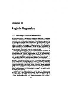
Figure 4: Display of C(fα , g0 ). x-axis: α. y-axis: C(fα , g0 ). Note that the Fourier coefficients of fα (θ) satisfy the decay condition in (5.2) with λ = 2−α. Also, we have the following lemma, which is derived in Section 12. Lemma 7.2 For 0 < α < 1, we have essinf −π≤θ≤π {fα (θ)} > 0. Next, let g0 (θ) = 1 − e−iθ ,

an = an (α0 ) = nα0 /2.

The Toeplitz matrix Σn (g0 ) is a lower triangular matrix with 1’s on the main diagonal, −1’s on the sub-diagonal, and 0’s elsewhere. Additionally, let Dn be the diagonal matrix where on √ ˜ = Dn · Σn (g0 ) · X. the diagonal the first entry is 1 and the remaining entries are an . Let X Then Model (7.1) can be rewritten equivalently as ˜ =µ ˜ n ), X ˜ + Z˜ where µ ˜ = Dn · Σn (g0 ) · µ and Z˜ ∼ N(0, Σ

(7.3)

˜ n = Dn · Σn (g0 ) · Σn · Σn (¯ ˜ n is asymptotically equivalent with Σ g0 ) · Dn . The key is that Σ to the Toeplitz matrix generated by fα . In detail, introduce   1, 0 ¯= Σ . 0, Σn−1 (fα ) The following lemma is proved in Section 11. ˜n − Σ ¯ n tends to 0 as n tends to ∞. Lemma 7.3 The spectral norm of Σ √ Additionally, note that µ ˜ = an · Σn−1 (g) · µ except for the first coordinate. Therefore, we expect Model (7.3) to be approximately equivalent to ˜ = √an · Σn (g0 ) · µ + Z˜ where Z˜ ∼ N(0, Σn (fα )). X This is a special case of the cluster model we considered in Section 6 with f = fα and g = g0 , √ except that the signal strength has been re-scaled by an . Therefore, if we calibrate the nonzero entries in µ as p −1/2 a−1/2 · A = a · 2r log n, (7.4) n n n

14

then the detection boundary for the model is succinctly characterized by Z π Z |g0 (θ)|2 1 1 1 π 1 − cos(θ) ∗ r= · ρ (β), C(fα , g0 ) = dθ = dθ . C(fα , g0 ) 2π −π fα (θ) π −π fα (θ) See Figure 4 for the display of C(fα , g0 ). The following theorem is proved in Section 10. Theorem 7.1 Let 0 < α0 ≤ α < 12 , β ∈ ( 12 , 1), and r ∈ (0, 1). Assume X is generated according to Model (7.1), with signal strength re-scaled as in (7.4). When C(fα , g0 ) · r < ρ∗ (β), the null and alternative hypotheses merge asymptotically, and the sum of Type I and Type II errors of any test converges to 1 as n diverges to ∞. When C(fα , g0 ) · r > ρ∗ (β), if we apply the iHC to X with bandwidth bn = log n and reject the null when iHCn∗ (bn , Σn ) ≥ (log n)2 , then the Type I error converges to zero, and its power converges to 1. 0.3

0.3

0.25

0.25

0.2

0.2

0.15

0.15

0.1

0.1

0.05

0.05

0

−0.4

−0.2

0

0.2

0

0.4

0.3

0.3

0.25

0.25

0.2

0.2

0.15

0.15

0.1

0.1

0.05

0.05

0

−0.4

−0.2

0

0.2

0

0.4

−0.4

−0.2

0

0.2

0.4

−0.4

−0.2

0

0.2

0.4

Figure 5: Sum of Type I and Type II errors as described in experiment (a). From top to bottom then from left to right, (β, r) = (0.5, 0.2), (0.5, 0.25), (0.55, 0.2), (0.55, 0.25). In each panel, the x-axis displays ρ, and three curves (blue, dashed-green, and red) display the sum of errors corresponding to HC, HC-a, and HC-b.

8

Simulation study

We conducted a small-scale empirical study to compare the performance of iHC and standard HC. For iHC, we investigate two choices of bandwidth: bn = 1 and bn = log n. In this section, we denote standard HC, iHC with bn = 1, and iHC with bn = log n by HC, HC-a, and HC-b correspondingly. The algorithm for generating√data included the following four steps: (1). Fix n, β, and r, let m = n1−β and An = 2r log n. (2). Given a correlation matrix Σn , generate a Gaussian vector Z ∼ N(0, Σn ). (3). Randomly draw m integers `1 < `2 < . . . < `m from {1, 2, . . . , n} without replacement, and let µ be the n-vector such that µj = An if j ∈ {`1 , `2 , . . . , `m } and 0 otherwise. (4). Let X = µ + Z. Using data generated in this manner we explored three parameter settings, (a)–(c), which we now describe. 15

In experiment (a), we took n = 1000 and Σn (ρ) as the tri-diagonal Toeplitz matrix generated by f (θ) = 1 + 2ρ cos(θ), |ρ| 0 such that kU k ≤ C ˜ 0U ˜ −U ˜ 0U ˜ k = kW 0 W + U ˜ 0W + W 0U ˜ k ≤ CkW k. Moreover, by and kW k ≤ C, whence kU [22, Theorem 5.6.9], for any symmetric matrix, the spectral norm is no greater than the `1 -norm. In view of the definitions of W and Θ∗n (λ, c0 , M ), the `1 -norm of W is no greater ˜ 0U ˜ −U ˜ 0U ˜ k ≤ CkW k ≤ C(log n)−2(λ−1) . This, and the than (log n)−2(λ−1) . Therefore, kU ˜ 0U ˜ are bounded from below by a positive constant, imply the fact that all eigenvalues of U claim. We now consider the second claim. Model (10.2) can be equivalently written as X = ˜ ˜ is a banded matrix and µ Uµ ˜ + Z where Z ∼ N(0, In ). The key to the proof is that U is a sparse vector where with probability converging to 1, the inter-distances of nonzero coordinates are no less than 3(log n)2 (see Lemma 11.2 for the proof). As a result the ˜µ nonzero coordinates of U ˜ are disjoint clusters of sizes O(log2 n), which simplifies the calculation of the Hellinger distance. The derivation of the claim is lengthy, so we summarize it in the following lemma, which is proved in Section 11. Lemma 10.1 Fix β ∈ ( 12 , 1), r ∈ (0, 1), and δ ∈ (0, 1) such that γ¯0 (1 − δ)−2 r < ρ∗ (β). As n tends to ∞ the Hellinger distance associated with Model (10.2) tends to 0.

10.3

Proof of Theorem 4.1

Put Y = Un (Σn )X, ν = Un (Σn )µ, and Z = Un (Σn )z. Model (4.1) reduces to Z ∼ N(0, In ).

Y = ν + Z,

(10.3)

√ Recalling that HCn∗ / 2 log log n → 1 in probability under H0 , it follows that PH0 {Reject H0 } tends to 0 as n diverges to ∞, and it suffices to show PH (n) {Accept H0 } → 0. 1

The key to the proof is to compare Model (10.3) with Y ∗ = ν∗ + Z

where

Z ∼ N(0, In ),

(10.4)

with ν ∗ having m nonzero entries of equal strength (1−δn )An whose locations are randomly ˜ ∗n (δn , bn ) is drawn from {1, 2, . . . , n} without replacement. By (4.2)–(4.3) and the way Θ defined, we note that νj ≥ (1 − δn )An for all j ∈ {`1 , `2 , . . . , `m }. Therefore, signals in ν is both denser and stronger than those in ν ∗ .

(10.5)

Intuitively, standard HC applied to Model (10.3) is no “less” than that applied to Model (10.4). We now establish this point. Let F¯0 (t) be the survival function of the central χ2 distribution χ21 (0), and let F¯n (t) and F¯n∗ be the empirical survival function of {Yk2 }nk=1 and {(Yk∗ )2 }nk=1 , respectively. Using arguments similar to those of Donoho and Jin [14] it can (1) be shown that standard HC applied to Models (10.3) and (10.4), denoted by HCn and (2) HCn for short, can be rewritten as √ ¯  n(Fn (t) − F¯0 (t)) (1) p HCn = sup , F¯0 (t)F0 (t) {t: 1/n≤F¯0 (t)≤1/2} HCn(2)

√ =

sup {t: 1/n≤F¯0 (t)≤1/2}

20

 n(F¯n∗ (t) − F¯0 (t)) p , F¯0 (t)F0 (t)

respectively. The key fact is now that the family of non-central χ2 -distribution {χ21 (δ), δ ≥ 0} is a monotone likelihood ratio family (MLR), i.e. for any fixed x and δ2 ≥ δ1 ≥ 0, P {χ21 (δ2 ) ≥ x} ≥ P {χ21 (δ1 ) ≥ x}. Consequently, it follows from (10.5) and mathematical induction that for any x and t, P {F¯n∗ (t) ≥ x} ≥ P {F¯n (t) ≥ x}. Therefore, for any fixed x > 0, P {HCn(1) < x} ≤ P {HCn(2) < x}. (10.6) Finally, by an argument similar √ to that of Donoho and Jin [14, Section 5.1], the second term in (10.6) with x = 1.01 2 log log n tends to 0 as n diverges to ∞. This implies the claim. 

10.4

Proof of Theorem 4.2

¯ =U ¯ (bn ), In view of Lemma 4.2, it suffices to show that PH (n) {Accept H0 } → 0. Put U 1 V = Vn (bn ), Y = V X, ν = V µ, Z˜ = V Z. Model (4.7) reduces to Y = ν + Z˜

where

¯ 0U ¯ ). Z˜ ∼ N(0, U

(10.7)

Let F¯n (t) and F¯0 (t) be the empirical survival function of {Yk2 }nk=1 and the survival func2 Let q = q(β, r) = min{(β + γ¯0 r)2 /(4¯ γ0 r), 4¯ γ0 r} and set t∗n = tion √ of χ1 (0), respectively. ∗ 2q log n. Since γ¯0 r < ρ (β), then it can be shown that 0 < q < 1 and n−1 ≤ F¯0 (t∗n ) ≤ 1/2 for sufficiently large n. Using an argument similar to that in the proof of Theorem 4.1, √ ¯ √ ¯ ∗ n(Fn (s) − F¯0 (s)) n(Fn (tn ) − F¯0 (t∗n )) ∗ p iHCn = sup ≥p , (2bn − 1)F¯0 (s)(1 − F¯0 (s)) (2bn − 1)F¯0 (t∗n )(1 − F¯0 (t∗n )) {s: 1/n≤F¯0 (s)≤1/2} and it follows that √ ¯ ∗ n(Fn (tn ) − F¯0 (t∗n )) P {iHCn∗ ≤ log3/2 (n)} ≤ P { p ≤ log3/2 (n)}. ∗ ∗ ¯ ¯ (2bn − 1)F0 (tn )(1 − F0 (tn ))

(10.8)

It remains to show that the right hand side of (10.8) is algebraically small. The proof needs detailed calculation which we summarize in the lemma below, the proof of which is given in Section 11. Lemma 10.2 Under the condition of Theorem 4.2, the right hand side of (10.8) tends to 0 algebraically fast as n diverges to ∞.

10.5

Proof of Theorem 6.1

Inspection of the proof of Theorems 3.2 and 4.2 reveals that the condition that Σn is a correlation matrix and that Σn ∈ Θ∗n (λ, c0 , M ) in those theorems can be relaxed. In particular, Σn need not have equal diagonal entries and the decay condition on Σn can be replaced by a weaker condition that concerns the decay of Un (the inverse of the Cholesky factorization of Σn ), specifically |Un (i, j)| ≤ M (1 + |i − j|λ )−1 . ˜n = Let Un (f ) be the inverse of the Cholesky factorization of Σn (f ), and define U Un (f )Σn (g). Since Σn (g) is a lower triangular matrix with positive diagonal entries, then ˜n is the inverse of the Cholesky factorization of Σ ˜ n . By Lemma 3.2, Un (f ) it is seen that U 21

˜n decays at the has polynomial off-diagonal decay with the parameter λ. It follows that U same rate. Applying Theorems 3.2 and 4.2, we see that all that remains to prove is that ˜ −1 √ max √ {|Σn (k, k) { n≤k≤n− n} By [5, Theorem 2.15], for any

√

n≤k ≤n−

− C(f, g)|} → 0.

√

(10.9)

n, k − K ≤ j ≤ k + K, and 1 ≤ λ0 < λ, 0

−(1−λ )/2 |Σ−1 ). n (f )(k, j) − (Σn (1/f ))(k, j)| = o(n √ √ ˜ −1 ˜ −1 Since Σ g ) · Σ−1 g) · n = Σn (¯ n (f ) · Σn (g), it follows that sup{ n≤k≤n− n} |Σn (k, k) − (Σn (¯ Σn (1/f ) · Σn (g))(k, k)| → 0. Moreover, direct calculations show that (Σn (¯ g ) · Σn (1/f ) · √ √ Σn (g))(k, k) = C(f, g), n ≤ k ≤ n − n. Combining these results gives (10.9) and concludes the proofs. 

10.6

Proof of Theorem 7.1

˜ and Z˜ Consider the first claim. It suffices to show that the Hellinger distance between X ∗ in Model (7.3) tends to 0 as n diverges to ∞. Since C(fα , g0 ) · r < ρ (β), there is a small constant δ > 0 such that (1 − δ)−1 · C(fα , g0 ) · r < ρ∗ (β). Using Lemma 7.2, we see that Σn−1 (fα ) is a positive matrix the smallest eigenvalue of which is bounded away from 0. ˜ ≥ (1 − δ)Σ ¯ n for sufficiently large n. It follows from Lemma 7.3 and basic algebra that Σ Compare Model (7.3) with X∗ = µ ˜ + Z∗

where

¯ Z ∗ ∼ N(0, (1 − δ)Σ).

(10.10)

By the monotonicity of Hellinger distance (Theorem 3.1), it suffices to show that the Hellinger distance between X ∗ and Z ∗ tends to 0 as n diverges to ∞. √ √ Now, by the definition of µ ˜, µ ˜ − an · Σn (g0 ) · µ = (µn , an · µn , 0, . . . , 0)0 . Since P {µn 6= 0} = o(1) then, except for an event with negligible probability, µ ˜=µ ¯. Therefore, √ replacing µ ˜ by an · Σn (g0 ) · µ in Model (10.10) alters the Hellinger distance only negligibly. Note that the first coordinate of X ∗ is uncorrelated with all other coordinates, and its mean equals 0 with probability converging to 1, so removing it from the model only has a negligible effect on the Hellinger distance. Combining these properties, Model (10.10) reduces to the following with only a negligible difference in the Hellinger distance: √ X ∗ (2 : n) = Σn−1 (g0 )( an · µ(2 : n)) + Z ∗ (2 : n),

Z ∗ (2 : n) ∼ N(0, (1 − δ)Σn−1 (fα )),

where X(2 : n) denotes the vector X with the first entry removed. Dividing both sides by √ 1 − δ, this reduces to the following model: √ an · µ(2 : n)
˜ ˜ ˜ : n) ∼ N(0, Σn−1 (fα )), (10.11) √ X(2 : n) = Σn−1 (g0 ) + Z(2 : n), Z(2 1−δ √ which is in fact Model (6.1) considered in Section 6. It follows p from (7.4) that an · µ(2 : √ n)/ 1 − δ has m nonzero coordinates each of which equals 2(1 − δ)−1 r log n. Comparing Model (10.11) with Model (6.1) and recalling that (1 − δ)−1 · r · C(fα , g0 ) < ρ∗ (β), the claim follows from Theorem 6.1. Consider the second claim. Since C(fα , g0 ) · r > ρ∗ (β), then there is a small constant δ > 0 such that (1 − δ) · r · C(fα , g0 ) > ρ∗ (β). Let Un be the inverse of the Cholesky

22

¯n (bn ) and Vn (bn ) be as defined right below (4.5). Write Model factorization of Σn , and let U (7.1) equivalently as VX =Vµ+VZ

¯ 0 (bn )U ¯ (bn )). where V Z ∼ N(0, U

¯ 0 (bn )U ¯ (bn ) is a banded correlation matrix with bandwidth 2bn − 1. Let Recall that U `1 , `2 , . . . , `m be the m locations of nonzero means of µ. By an argument similar to that in the proof of Theorem 4.2, all remains to show is that, except for an event with negligible probability, p (V µ)k ≥ 2r0 log n for some constant r0 > ρ∗ (β) and all k ∈ {`1 , `2 , . . . , `k }. (10.12) We now show (10.12). First, by Lemma 4.1 and (7.4), except for an event with negligible probability, (V µ)k ≥ (1 − δ)1/4 · (an · Σn (k, k))−1/2 · An ,

k ∈ {`1 , `2 , . . . , `m }.

˜ n is defined, Second, by the way Σ ˜ −1 (an Σ−1 g0 ))(k, k), n )(k, k) = (Σn (g0 ) · Σn · Σn (¯

for all k ≥ 2,

¯ n is defined and Lemma 7.3, for sufficiently large n, and by the way Σ ¯ −1 , and so Σn (g0 )Σ ˜ −1 Σn (¯ ¯ −1 Σn (¯ ˜ −1 ≥ (1 − δ)−1/2 Σ g0 ) ≥ (1 − δ)1/2 Σn (g)Σ g ). Σ n n n n ¯ −1 ·Σn (¯ Last, by [5, Theorem 2.15], |(Σn (g0 )· Σ g0 ))(k, k)−C(fα , g0 )| = o(1) when min{k, n− n k} is sufficiently large. Combining these results gives (10.12) with r0 = (1 − δ) · r · C(fα , g0 ), and the claim follows directly. 

11

Appendix

This section contains proofs for all lemmas in preceding sections, except Lemmas 3.1, 5.1, 7.1, and 7.2. Lemma 3.1 is the direct result of [35] and Lemma 5.1 is the direct result of [5, Theorem 2.15], so we omit the proofs. Lemmas 7.1 and 7.2 are proved in Section 12.

11.1

Proof of Lemma 3.2

Consider the first claim. Construct an infinite matrix Σ∞ by arranging the finite matrices along the diagonal, and note that the inverses of Σ∞ is the matrix formed by arranging the inverse of the finite matrices along the diagonal. Since Σ∞ (i, j) ≤ M (1 + |i − j|λ )−1 , then applying Lemma 3.1 gives the claim. Consider the second claim. It suffices to show that |Un (k, j)| ≤ C/(1 + |k − j|λ ) for all 1 ≤ j < k ≤ n. Denote the first k × k main diagonal sub-matrix of Σn by Σk , the k-th row 0 of Σk by (ξk−1 , 1), and the k-th row of Un by u0k . It follows from direct calculations that 0 u0k = 1 − ξk−1 Σ−1 k−1 ξk−1


−1/2

0 · (ξk−1 Σ−1 k−1 , 1).

(11.1)

At the same time, by (11.1) and basic algebra, 0 1 − ξk−1 Σ−1 k ξk−1


−1

≤ u0k uk = Σ−1 k (k, k).

23

(11.2)

Combining (11.1) and (11.2) gives |Un (k, j)| = |uk (j)| ≤ C|(Σ−1 k−1 ξk−1 )j |,

1 ≤ j ≤ k − 1.

(11.3)

λ −1 for all 1 ≤ i, j ≤ k − 1. Note that Now, by Lemma 3.1, |Σ−1 k−1 (j, s)| ≤ C(1 + |j − s| ) λ −1 |ξk−1 (s)| ≤ C(1 + |s − k| ) , 1 ≤ s ≤ n, and λ > 1. It follows from basic algebra that

|(Σ−1 k−1 ξk−1 )j | ≤

n X s=1

C C ≤ . (1 + |j − s|λ )(1 + |s − k|λ ) 1 + |k − j|λ

Inserting (11.4) into (11.3) gives the claim.

11.2

(11.4) 

Proof of Lemma 4.1

Without loss of generality, assume `1 < `2 < . . . < `m . By Lemma 11.2, except for an event with negligible probability, `1 ≥ bn , `m ≤ n − bn , and the inter-distances of the `j ’s Pk+bn −1 2
−1/2 . By the way ujk ≥ C log n · n2β−1 . For any k ∈ {`1 , `2 , . . . , `m }, let dk = j=k ¯ (bn ) is defined, U ¯ 0 (bn )U µ)k = dk (U

n X

u ˜ks usj µj = dk

s,j=1

X n

uks usj µj −

s,j=1

n X

 (uks − u ˜ks )usj µj .

(11.5)

s,j=1

Consider dk first. Write 1/d2k =

k+b n −1 X

u2jk =

n X j=k

j=k

u2jk −

n X

u2jk .

j=k−bn

Pn 0 −1 2 First, U 0 U = Σ−1 , j=k ujk = (U U )(k, k) = (Σ )(k, k). Second, by the polynomial off-diagonal decay of U and basic calculus, n X

u2jk

j=k+bn

≤C

n X j=k+bn

1 ≤ Cb1−2λ . n 1 + |j − k|λ

Last, note that the quantities Σ−1 (k, k) are uniformly bounded away from 0 and ∞. Combining these results gives p (11.6) |dk − Σ−1 (k, k)| ≤ Cbn1−2λ . Pn Consider s,j=1 uks usj µj next. Recall that µj = An when j ∈ {`1 , `2 , . . . , `m } and µj = 0 otherwise. Since U 0 U = Σ−1 , n X s,j=1

uks usj µj =

n X

(Σ−1 )(k, j)µj = An Σ−1 (k, k) + An

X

Σ−1 (k, `s ).

`s 6=k

j=1

Define Ln = nβ−1/2 . By Lemma 11.2, except for an event with negligible probability, the inter-distance of `j is no less than Ln . So by the polynomial off-diagonal decay of Σ−1 , the second term is algebraically small. Therefore, n X

uks usj µj = An [(Σ−1 )(k, k) + o(bn1−λ )].

s,j=1

24

(11.7)

Last, we consider

Pn

−u ˜ks )usj µj . Direct calculations show that ( C , λ > 1, 1+|k−j|λ 0 ˜ |((U − U ) U )(k, j)| ≤ C log n , λ = 1, 1+|k−j|λ s,j=1 (uks

so by a similar argument, n n X X 0 ˜ ˜ )0 U )(k, k) + o(1), ≤ An · ((U − U (u − u ˜ )u µ = ((U − U ) U )(k, j)µ sj j j ks ks s,j=1

j=1

where o(1) is algebraically small. Moreover, by the Cauchy-Schwartz inequality, ˜ )0 U )(k, k) ≤ ((U − U

n X

|(uks − u ˜ks )usk | ≤ bn1/2−λ ,

s=1

and the claim follows.

11.3



Proof of Lemma 4.2

Without loss of generality, suppose n is divisible by 2bn − 1, and let N = N (n, bn ) = n/(2bn − 1). Let pi be N iid samples from U (0, 1), and FN (t) be the empirical cdf. The normalized uniform stochastic process is defined as p √ WN (t) = N [FN (t) − t]/ t(1 − t). The following lemma is proved in Section 11.3.1. Lemma 11.1 There is a generic constant C > 0 such that for sufficiently large n,  P sup |WN (t)| ≥ C(log n)3/2 ≤ Cn−C . {1/n≤t≤1/2}

¯ 0 U X. Under the null hypothesis, Y ∼ We now prove Lemma 4.2. Define Y = U 0 ¯U ¯ ) and the coordinates Yk are block-wise dependent with a bandwidth ≤ 2bn − 1. N(0, U Split the Yk ’s into 2bn −1 different subsets Ωj = {Yk : k ≡ j mod (2bn −1)}, 1 ≤ j ≤ 2bn −1. Note that the Yk ’s in each subset are independent, and that |Ωj | = N , 1 ≤ j ≤ 2bn − 1. Let F¯n (t) and F¯0 (t) be as in the proof of Theorem 4.1, and let n

2bn − 1 X 1{Y 2 ≥t, Yk ∈Ωj } , F¯n,j = k n

1 ≤ j ≤ 2bn − 1.

k=1

P n −1 ¯ Note that F¯n (t) = 2bn1−1 2b j=1 Fn,j (t). By arguments similar to that of Donoho and Jin [14], and basic algebra, it follows that iHCn∗

 √ ¯  2bX √  n −1 N (F¯n,j (t) − F¯0 (t)) n(Fn (t) − F¯0 (t)) p = sup p ≤ sup , t t (2bn − 1)F¯0 (t)F0 (t) F¯0 (t)F0 (t) j=1

and so for any x > 0, P {iHCn∗ ≥ x} ≤

2bX n −1 j=1

√   N (F¯n,j (t) − F¯0 (t)) p P sup ≥x . t F¯0 (t)F0 (t) 

25

Finally, since that F¯n,j ’s are the empirical survival functions of N independent samples from χ21 (0), then √  N (F¯n,j (t) − F¯0 (t)) p = sup {WN (t)} in distribution. sup F¯0 (t)F0 (t) {1/n≤t≤1/2} 1/n≤F¯0 (t)≤1/2 Therefore, P {iHCn∗ ≥ x} ≤ (2bn − 1)P {

sup

{WN (t)} ≥ x}.

{1/n≤t≤1/2}

Taking x = C(log n)3/2 , the claim follows from Lemma 11.1. 11.3.1



Proof of Lemma 11.1

By the Hungarian construction [10], there is a Brownian bridge B(t) such that P{

√ C(log N + x) √ | N (FN (t) − t) − B(t)| ≥ } ≤ Ce−Cx , N {1/n≤t≤1/2} sup

p √ √ where C > 0 are generic constants. Noting that 1/ t(1 − t) ≤ n ≤ C N log N when 1/n ≤ t ≤ 1/2, it follows that √   N (FN (t) − t) − B(t) 1/2 ≥ C(log N ) (log N + x) ≤ Ce−Cx . p P sup (11.8) t(1 − t) {1/n≤t≤1/2} At the same time, by [33, Page 446],   B(t) 1/2 −Cx P sup . pt(1 − t) ≥ C(log N ) x ≤ C log N · e {1/n≤t≤1/2}

(11.9)

Combining (11.8)–(11.9), taking x = C log N and using triangle inequality, gives the claim. 

11.4

Proof of Lemma 7.3

˜ is defined, we have By direct calculations and the way Σ  ∗  Σ ξn−1 ˜ Σ= , 0 ξn−1 1

(11.10)

where 0 ξn−1 =

√

2n−α × (0, . . . , nα0 − k0 (n)α , k0 (n)α − (k0 (n) − 1)α , . . . , 2α − 1, 1)

(11.11)

and Σ∗ is a symmetric matrix with unit diagonal entries, and with the following on the k-th sub-diagonal:  2k α − (k + 1)α − (k − 1)α , k ≤ k0 (n) − 1,    1 1 + ((k − 1)α − 2k α )/nα0 = O(n−α0 /α ), k = k0 (n), · −(1 − (k − 1)α /nα0 ) = O(n−α0 /α ), k = k0 (n) + 1, 2    0, k ≥ k0 (n) + 2.

26

Note that Σn−1 (g0 ) and Σ∗ share the same 2k0 (n) − 1 sub-diagonals that are closest to the main diagonal (including the main diagonal). Let H1 be the matrix containing all other sub-diagonals of Σn−1 (g0 ), and let H2 be the the matrix which contains the k0 (n)-th and the (k0 (n) + 1)-th diagonals (upper and lower) of Σ∗ . It is seen that       0 H1 0 H2 0 0 ξn−1 ˜ ¯ Σ−Σ= + + ≡ B1 + B2 + B3 . 0 0 0 0 0 ξn−1 0 Let k · k1 and k · k2 denote the `1 matrix norm and the `2 matrix norm, respectively. First, by direct calculations, since α < 1/2, kB1 + B2 k1 ≤ Cnα0 (α−1)/α ≤ Cn−α0 . At the same time, by (11.11) and since α < 1/2, n n C X α C X 2α−2 α 2 kB3 k ≤ α0 (k − (k + 1) ) ≤ α0 k ≤ C/nα0 . n n 2

k=1

k=1

Since the spectral norm is no greater than the `1 -matrix norm and the `2 -matrix norm, the spectral norm of B1 + B2 + B3 is no greater than Cn−α0 /2 , and the claim follows. 

11.5

Proof of Lemma 10.1

p ˜ , and µ ˜˜ = γ0 , r0 = γ¯0 (1 − δ)−2 r, U1 = aU Let a = (1 − δ)/¯ equivalently written as ˜µ ˜˜ + Z X=U ˜ + Z = U1 µ

where

1 ˜. aµ

Model (10.2) can be

Z ∼ N(0, In ).

(11.12)

Using the argument in the first paragraph of the proof of Theorem√3.2 it is not hard to verify ˜ that (I) µ ˜ has m = n1−β nonzero entries each of which is equal to 2r0 log n with r0 < ρ∗ (β), and whose locations are randomly sampled from (1, 2, . . . , n); (II) U1 , where U1 (k, j) = 0 if |k − j| > (log n)2 , is a banded lower triangular matrix; and (III) limn→∞ max{√n≤k≤n−√n} {(U10 U1 )(k, k)} = (1 − δ) < 1. 0 ˜ From now on, write µ = µ ˜ and p r = r for short. Note that the Hellinger affinity ∗ associated with Model (10.2) is E0 ( Wn ), where E0 denotes the law Z ∼ N(0, In ), and  −1 X n 0 0 2 ∗ ∗ eµ` U1 Z−kU1 µ` k /2 . Wn = Wn (r, β; Z1 , Z2 , . . . , Zn ) = m {`=(`1 ,`2 ,...,`m )}

Introduce the set of indices  Sn = ` = (`1 , `2 , . . . , `m ),

min

{1≤j≤m−1}

|`j+1 − `j | ≥ 3(log n)2 , `1 ≥

√

n, n − `m ≥

√ n . (11.13)

The following lemma is proved in Section 11.5.1. Lemma 11.2 Let `1 < `2 < . . . < `m be m distinct indices randomly sampled from (1, 2, . . . , n) without replacement. Then for any 1 ≤ K ≤ n, (a) P {`1 ≤ K} ≤ Km/n, (b) P {`m ≥ n − K} ≤ Km/n, and (c) P {min{1≤i≤m−1} {|`i+1 − `i | ≤ K} ≤ Km(m + 1)/n. As a result, P {` = (`1 , `2 , . . . , `m ) ∈ / Sn } = O{(log n)2 n1−2β } = o(1). Applying Lemma 11.2, we make only a negligible difference by restricting ` to Sn and defining X 1 0 0 2 eµ` U1 Z−kU1 µ` k /2 , (11.14) Wn = n
m

{`=(`1 ,`2 ,...,`m )∈Sn }

27

in which case E(Wn1/2 ) = E(Wn∗ 1/2 ) + o(1). Define Y =

U10 Z,

σj2 = var(Yj ) ≡ (U10 U1 )(j, j),

(11.15)

1 ≤ j ≤ n,

(11.16)

and the event Dn = {Yj /σj ≤

p 2 log n, 1 ≤ j ≤ n}. 1/2

By direct calculation, P {Dnc } = o(1), and so by H¨older’s inequality, E(Wn 1/2 E(Wn )+o(1).

1{Dnc } ) =

E(Wn∗ 1/2 )

1/2

Combining this result and (11.15) we deduce that = E(Wn 1{Dn } )+ o(1), and comparing this property with the desired result we see that it is is sufficient to show that E(Wn1/2 1{Dn } ) = 1 + o(1). (11.17) The key to (11.17) is the following lemma, which is proved in Section 11.5.2. Lemma 11.3 Consider Model (11.12), where U1 and µ satisfy (I)–(III). As n → ∞, E(Wn 1{Dn } ) = 1 + o(1), and E(Wn2 1{Dn } ) = 1 + o(1). Since |Wn1/2 1{Dn } − 1| ≤

|Wn 1{Dn } − 1| 1/2

1 + Wn

1{Dn }

≤ |Wn 1{Dn } − 1|,

then by H¨ older’s inequality, 2
2

E|Wn1/2 1{Dn } − 1| ≤ Wn 1{Dn } − 1 = E Wn2 1{Dn } − 2E Wn 1{Dn } + 1.

(11.18)

Combining (11.18) with Lemma 11.3 gives (11.17). 11.5.1



Proof of Lemma 11.2

The last claim follows once (a)–(c) are proved. Consider (a)–(b) first. Fixing K ≥ 1,
n−K (n − m)(n − m − 1) . . . (n − m − K + 2) m−1
=m P {`1 = K} = ≤ m/n, n n(n − 1) . . . (n − K + 1) m so P {`1 ≤ K} ≤ Km/n. Similarly, P {n − `m ≤ K} ≤ Km/n. This gives (a) and (b). Next we prove (c). Denote the minimum inter-distance of `1 , `2 , . . . , `m by L(`) = L(`; m, n) = min{1≤i≤m−1} {|`i+1 − `i |}. Note that P {L(`) = K} ≤

m−1 X

m−1 n XX

j=1

j=1 k=1

{`j+1 − `j = K} ≤

Writing P {`j = k, `j+1 = k + K} = P {L(`) = K} ≤

P {`j = k, `j+1 = k + K}.




n −1 k−1 n−k−K m j−1 m−j−1 ,

we have:

    m−1 n  n k  1 XX k−1 n−k−K 1 XX k − 1 n − k − K

= , n n j−1 m−j−1 j−1 m−j−1 m m j=1 k=j

k=1 j=1

where the last term is no greater than  n  1 X n−K −1
≤ n m−2 m k=1

and the claim follows.

 n
≤ m2 /n, n−2 m − 2 m n



 28

11.5.2

Proof of Lemma 11.3 √ Define Tn = 2 log n. We need the following lemma, which is proved in Section 12. Lemma 11.4 Consider a bivariate zero mean normal variable (X, Y )0 that satisfies Var(X) = σ12 , Var(Y ) = σ22 , and corr(X, Y ) = %, where c0 ≤ σ1 , σ2 ≤ 1 for some constant c0 ∈ (0, 1). Then there is a constant C > 0 such that for sufficiently large n, √ 2 √ 2 
 E exp An X − σ12 A2n /2 · 1{Y /σ2 >Tn } ≤ C · n−(1−% r) ≤ Cn−(1− r) ,   σ 2 + σ22 2
E exp An (X + Y ) − 1 An · 1{X/σ1 ≤Tn ,Y /σ2 ≤Tn } ≤ Cn−d(r) , 2 √ 2 where d(r) = min{2r, 1 − 2(1 − r) }. We also need the following definition. Definition 11.1 We say that two indices j and k are near to each other if |j−k| ≤ (log n)2 . We now proceed to show Lemma 11.3. Consider the first claim. Note that for any ` = (`1 , `2 , . . . , `m ) ∈ Sn , the minimum inter-distance of `i is no less than 3(log n)2 . In view of the definition of Yj and σj (see (11.16)), we have kU1 µ` k2 = A2n

m X

(U10 U1 )(`i , `i ) = A2n

i=1

m X

σ`2i .

i=1

Consequently, we can rewrite Wn as 1

X

m

`=(`1 ,`2 ,...,`m )∈Sn

Wn = n
Note that

1

c} {Dn

≤

 X  m m A2n X 2 exp An Y`i − σ`i . 2 i=1

n X

(11.19)

i=1

1{Yj /σj >Tn } .

(11.20)

j=1

Combining (11.19) and (11.20) gives 1

X

E[Wn · 1{Dnc } ] ≤ n
m

  X   n m m X A2n X 2 E exp An Y`j − σ`j · 1{Yk /σk >Tn } . 2 j=1

`=(`1 ,...,`m )∈Sn k=1

j=1

(11.21) Now, for each 1 ≤ k ≤ n, when k is near one `j , say `j0 , Yk must be independent of all other Y`j with j = 6 j0 . It follows that   X   m m 
 A2 X 2 E exp An Y`j − n σ`j · 1{Yk /σk >Tn } = E exp An Y`j0 − σj20 A2n /2 · 1{Yk /σk >Tn } . 2 j=1

j=1

By Lemma 11.4, the right hand side is no greater than Cn−(1−

√

r)2 .

Therefore,

 X   m m √ 2 A2n X 2 E exp An Y`j − σ`j · 1{Yk /σk >Tn } ≤ Cn−(1− r) . 2 

j=1

j=1

29

(11.22)

Moreover, for each fixed ` = (`1 , . . . , `m ) ∈ Sn , there are at most 2m(log n)2 different indices k that can be near some of the `j ’s; and when they are, they can be near only one such `j . Combining these results gives X √ 2 √ 2 1 C(log n)2 mn−(1− r) ≤ C(log n)2 n(1−β)−(1− r) . E[Wn · 1{Dnc } ] ≤ n
m

`=(`1 ,...,`m )∈Sn

ρ∗ (β)

ρ∗ (β)

√ (11.23) ≤ (1 − 1 − β)2 ,

By the definition of and the assumption of the lemma, r < and so the first claim follows directly from (11.23). We now consider the second claim. Fix 0 ≤ N ≤ m, and let S˜N (`) denote the set of all k = (k1 , k2 , . . . , km ) ∈ Sn such that there are exactly N kj ’s that are near to one `i . (Clearly, any kj can be near to at most one `i ). The two sets of indices (`1 , `2 , . . . , `m ) and (k1 , k2 , . . . , km ) form exactly N pairs, each contains one candidate from the first set and one candidate from the second. These pairs are not near to each other, and not near to any remaining indices outside the pairs. Using (11.19), we write  −2 m X X X n 2 E[Wn · 1{Dn } ] = m `=(`1 ,`2 ,...,`m )∈Sn N =0 k=(k1 ,k2 ,...,km )∈S˜N (`)





× E exp An

m X i=1

  m A2n X 2 2 (Y`i + Yki ) − (σ`i + σki ) · 1{Dn } . 2

(11.24)

i=1

For any fixed ` and k ∈ S˜N (`), by symmetry, and without loss of generality, we suppose the N pairs are (`1 , k1 ), (`2 , k2 ), . . . , (`N , kN ). By independence of the pairs with other indices, and also by independence among the pairs,   X   m m A2n X 2 2 E exp An (Y`j + Ykj ) − (σ`j + σkj ) · 1{Dn } 2 j=1 j=1     X m m A2n X 2 2 ≤ E exp An (σ`j + σkj ) · 1{Y` /σ` ≤Tn ,Yk /σk ≤Tn , for all 1 ≤ j ≤ N } (Y`j + Ykj ) − j j j j 2 j=1

j=1

 X   N N A2n X 2 2 ≤ E exp An (Y`j + Ykj ) − · 1{Y` /σ` ≤Tn ,Yk /σk ≤Tn , for all 1 ≤ j ≤ N } (σ`j + σkj ) j j j j 2 j=1 j=1      A2n 2 N 2 = Πj=1 E exp An (Y`j + Ykj ) − (σ + σkj ) · 1{Y` /σ` ≤Tn ,Yk /σk ≤Tn . (11.25) j j j j 2 `j 

Here, in the first inequality, we have used the fact that 1{Dn } ≤ 1{Y`

j

/σ`j ≤Tn ,Ykj /σkj ≤Tn , for

all 1 ≤ j ≤ N } ;

in the second inequality, we have utilized the independence and the fact that
E[exp An Yj − σj2 A2n /2 ] = 1, for all j = 1, . . . , n; and in the third equality, we have used again the independence. Moreover, in view of the way U1 is defined and Lemma 3.2, there is a constant c0 ∈ (0, 1) such that σj ∈ [c0 , 1]. Using Lemma 11.4, for sufficiently large n and each 1 ≤ j ≤ N ,     A2n 2 2 (σ + σkj ) · 1{Y` /σ` ≤Tn ,Yk /σk ≤Tn ≤ Cnd(r) , (11.26) E exp An (Y`j + Ykj ) − j j j j 2 `j 30

with d(r) being as in Lemma 11.4. Combining (11.25) and (11.26) gives E[Wn2 · 1{Dn } ] ≤

 −2 n m

X

m X

(Cnd(r) )N S˜N (`) .

(11.27)

`=(`1 ,...,`m ) N =0

where |S˜N (`)| denote the cardinality of S˜N (`). By elementary combinatorics,        m n−N m n |S˜N (`)| ≤ (2 log2 n)N ≤ (2 log2 n)N . N m−N N m−N

(11.28)

Direct calculations show that
n
m N

m−N
n m

 2 m! 1 (n − m)! 1 m2
N = . . N ! (m − N )! (n − m + N )! N! n

(11.29)

Substituting (11.28)-(11.29) into (11.27) and recalling that m = n1−β , we deduce that E[Wn2 · 1{Dn } ] ≤

 −1 n m

where the last term ≤

X

(11.30)

`=(`1 ,`2 ,...,`m )∈Sn N =0

P∞

1 N =0 N !

∗

 N m X 1 m2
N (C log2 n)nd(r) , N! n

C log2 n)n1+d(r)−2β



r < ρ (β) =

β − 1/2, √ (1 − 1 − β)2 ,


N

. By the assumption of the lemma, 1/2 < β ≤ 3/4, 3/4 ≤ β < 1,

thus it can be seen that 1 + d(r) − 2β < 0 for all fixed β and r ∈ (0, ρ∗ (β)). Combining this with (11.30) gives the second claim. 

11.6

Proof of Lemma 10.2

The key observation is that, there is a sequence of positive numbers δn that tends to 0 as n diverges to ∞ such that νk ≥ (1 − δn )An for all k ∈ {`1 , `2 , . . . , `m }, so it is natural to compare Model (10.7) with the following model: Y ∗ = ν ∗ + Z,

Z ∼ N(0, In ),

(11.31)

where ν ∗ has m nonzero entries of equal strength (1 − δn )An whose locations are randomly drawn from {1, 2, . . . , n} without replacement. For short, write t = t∗n and √ ¯ n(Fn (t) − F¯0 (t)) Hn (t) = p . (2bn − 1)F¯0 (t)(1 − F¯0 (t)) Let F¯n∗ (t) be the empirical survival function of {(Yk∗ )2 }nk=1 , and let F¯ (t) = E[F¯n (t)] and F¯ ∗ (t) = E[F¯n∗ (t)]. Recall that the family of non-central χ2 -distributions has monotone likelihood ratio. Then F¯ (t) ≥ F¯ ∗ (t) ≥ F¯0 (t). Now, first, since the Yk ’s are block-wise dependent with a block size ≤ 2bn − 1, it follows by direct calculations that Var(Hn (t)) ≤ C F¯ (t)/F¯0 (t). Second, by F¯ (t) ≥ F¯n∗ (t), 31

√ ¯ √ ¯∗ n(F (t) − F¯0 (t)) n(F (t) − F¯0 (t)) E[Hn (t)] = p ≥p , (2bn − 1)F¯0 (t)(1 − F¯0 (t)) (2bn − 1)F¯0 (t)(1 − F¯0 (t))

(11.32)

where the right hand side diverges to ∞ algebraically fast, by an argument similar to that in [14]. Combine Chebyshev’s inequality, the identity bn = log n, and the calculations of the mean and variance of Hn (t), P {Hn (t) ≤ (log n)2 } ≤ C(log n)

F¯ (t)
2 . n F¯ (t) − F¯0 (t)

(11.33)

It remains to show that the last term in (11.33) is algebraically small. We discuss separately the cases F¯ (t)/F¯0 (t) ≥ 2 and F¯ (t)/F¯0 (t) < 2. For the first case, F¯ (t) C C ≤ ≤ , 2 n(F¯ (t) − F¯0 (t)) nF¯ (t) nF¯0 (t) √ which is algebraically small since t = 2q log n and 0 < q < 1. For the second case, C F¯0 (t) C F¯0 (t) F¯ (t) ≤ ≤ , n(F¯ (t) − F¯0 (t))2 n(F¯ (t) − F¯0 (t))2 n(F¯ ∗ (t) − F¯0 (t))2

(11.34)

which is seen to be algebraically small by comparing it to the right hand side of (11.32). This concludes the claim. 

12 12.1

Complementary technical details Proof of Lemma 7.1

Consider the first claim. Suppose such an autoregression structure exists for α ≥ α0 > 0. Let √ Yk = an · (Xk+1 − Xk )/d, an = nα0 /2, k = 1, 2, . . . , n − 1. Clearly, var(Yk ) = 1. At the same time, direct calculations show that the correlation between Y1 and Yj+1 equals to ((j + 1)α + (j − 1)α − 2j α )/2 for all 1 ≤ j ≤ n − 2, which is no larger than 1. Taking j = 2 yields (3α + 1 − 2 · 2α )/2 ≤ 1, and hence α ≤ 2. P Consider the second claim. For any k ≥ 1, define the partial sum Sk (t) = 1+2 kj=1 (1− jα + nα0 ) cos(kt). By a well-known result in trigometrics [38], to show the positive-definiteness of Σn , it suffices to show that Sk0 +1 (t) ≥ 0 for all t ∈ [−π, π] and Sk0 +1 (t) > 0 except for a measure 0 set.

(12.1)

Here, k0 = k0 (n; α, α0 ) is the largest integer k such that k α ≤ nα0 . α We now show (12.1). By that in [38, Page 183], if we let a0 = 2, and aj = 2(1 − njα0 )+ , Pk0 −1 1 ≤ j ≤ n − 1, then Sk0 +1 (t) = j=0 (j + 1)∆2 aj Kj (t) + (k0 + 1)Kk0 (t)∆ak0 + Dn (t)ak0 +1 . Here, ∆aj = aj − aj+1 , ∆2 aj = aj + aj+2 − 2aj+1 , and Dj (t) and Kj (t) are the Dirichlet’s kernel and the Fej´er’s kernel, respectively, sin((j + 21 )t) Dj (t) = , 2 sin( 2t )

 2 sin( j+1 2 2 t) Kj (t) = , j + 1 2 sin( 2t ) 32

j = 0, 1, . . . .

(12.2)

α

)+ = 0. Also, by the monotonicity of In view of the definition of k0 , ak0 +1 = (1 − (k0n+1) α0 P 0 −1 (j + 1)∆2 aj Kj (t). {aj }, ∆ak0 = ak0 − ak0 +1 ≥ 0. Therefore, Sk0 +1 (t) ≥ kj=0 We claim that the sequence {a0 , a1 , . . . , an−1 } is convex. In detail, since α ≤ 1, the α sequence {j α } is concave. As a result, the sequence {(1 − njα0 )} is convex, and so is the α sequenced {(1 − njα0 )+ }. In view of the definition of aj , the claim follows directly. The convexity of aj ’s implies that ∆2 aj ≥ 0, 0 ≤ j ≤ n − 2. Therefore, Sk0 +1 (t) ≥ 0. This proves the first part of (12.1). We now prove the second part of (12.1). We discuss separately for two cases α < 1 and α = 1. In the first case, ∆a0 = nα1 0 (2 − 2α ) > 0 and K0 (t) = 12 . As a result, α 1 Sk0 +1 (t) ≥ 2−2 2nα0 > 0, and the claim follows. In the second case, ∆aj = nα0 (2j − j − k0 −1 k0 1 (j + 2)) = 0, and ∆ak0 −1 = (1 − nα0 ) − 2(1 − nα0 ) = nα0 (k0 + 1) − 1 > 0. Therefore, k0 +1 Sk0 +1 (t) ≥ (k0 + 1)( kn0α+1 0 − 1)Kk0 (t). Clearly, Sk0 +1 (t) can only assume 0 when ( 2 )t is a multiple of π. Since the set of such t has measure 0, the claim follows directly. 

12.2

Proof of Lemma 7.2

Let a0 = 2, and ak = 2k α − (k + 1)α − (k − 1)α , 1 ≤ k ≤ n − 1. Clearly, ak > 0 for all k, so fα (0; α) > 0. Furthermore, when θ 6= 0, by [38, Equation 1.7, Page 183], ∞ X fα (θ) = (ν + 1)[aν+2 + aν − 2aν+1 ]aν Kν (θ),

(12.3)

ν=0

where Kν (θ) is the Fej´er’s kernel as in (12.2). By the positiveness of the Fej´er’s kernel, all remains to show is that ak+1 + ak−1 − 2ak > 0, for all k ≥ 2. Define h(x) = (1 + 2x)α + (1 − 2x)α − 4(1 + x)α − 4(1 − x)α + 6, 0 ≤ x ≤ 1/2. By direct calculations, for all k ≥ 2, 2 2 1 1 1 ak+1 +ak−1 −2ak = −k α [(1+ )α +(1− )α −4(1+ )α −4(1− )α +6] = −k α h( ). (12.4) k k k k k Also, by basic calculus, h00 (x) = 4α(α−1)[(1+2x)α−2 +(1−2x)α−2 −(1+x)α−2 −(1−x)α−2 ]. Since 0 < α < 1, xα−2 is a convex function. It follows that h00 (x) < 0 for all x ∈ (0, 1/2), and h(x) is a strictly concave function. At the same time, note that h(0) = h0 (0) = 0, so h(x) < 0 for x ∈ (0, 1/2]. Combining this with (12.4) gives the claim. 

12.3

Proof of Lemma 11.4

¯ For the first claim, Denote the density, cdf and survival function of N(0, 1) by φ, Φ, and Φ. define W = X/σ1 and V = Y /σ2 if ρ ≥ 0 and V = −Y /σ2 otherwise. The proofs for two cases ρ ≥ 0 and ρ < 0 are similar, so we only show the first one. In this case, it suffices to show √ 2 
 E exp σ1 An W − σ12 A2n /2 · 1{V >Tn } ≤ C · n−(1−% r) . Write W = (W − ρV ) + ρV , and note that (1 − ρ)2 + ρ2 ≤ 1. It is seen that σ1 An W − σ12 A2n /2 ≤ [σ1 An (W − ρV ) − σ12 (1 − ρ)2 A2n /2] + [σ1 An ρV − σ12 ρ2 A2n /2]. (12.5) Since W and V have unit variance and a correlation ρ, then (W − ρV ) is independent of V and is distributed as N(0, (1−ρ)2 ). Therefore, E[exp(σ1 An (W −ρV )−σ12 (1−ρ)2 A2n /2)] = 1. Combining this with (12.5) gives 
 
 E exp σ1 An W − σ12 A2n /2 · 1{V >Tn } = E exp σ1 ρAn V − σ12 ρ2 A2n /2 · 1{V >Tn } . 33

Now, by direct calculations, 
 E exp An V − A2n /2 · 1{V >Tn } =

Z

∞

¯ n − σ1 ρAn ). φ(x − σ1 ρAn )dx = Φ(T

Tn √

¯ ¯ n −σ1 ρAn ) ≤ Cφ(Tn −σ1 ρAn ) = Cn−(1−ρ r)2 . Combining Since Φ(x) ≤ Cφ(x) if x > 0, Φ(T these results gives the claim. We now show the second claim. By H¨older’s inequality, it suffices to show that E[exp(2An X − σ12 A2n ) · 1{X≤σ1 Tn } ] ≤ Cn−d(r) . Recalling that W = X/σ1 , we have E[exp(2An X − σ1 A2n ) · 1{X≤σ1 Tn } ] = E[exp(2σ1 An W − σ12 A2n ) · 1{W ≤Tn } ]. By direct calculations, E[exp(2σ1 An W −

σ12 A2n )

· 1{W ≤Tn } ] = e

σ12 A2n

Z

Tn

2

−∞

Since Φ(x) ≤ Cφ(x) for all x < 0 and Φ(x) ≤ 1 for all x ≥ 0, ( 2 2 2 2 2 Ceσ1 An = Cn2σ1 r , σ1 An √ 2 e Φ(Tn − 2σ1 An ) ≤ 2 2 eσ1 An φ(Tn − 2σ1 An ) = Cn1−2(1−σ1 r) , 2

2

φ(x − 2σ1 An )dx = eσ1 An Φ(Tn − 2σ1 An ).

2

σ12 r ≤ 1/4. σ12 r > 1/4;

2

in view of the definition of d(r), eσ1 An Φ(Tn − 2σ1 An ) ≤ Cnd(σ1 r) . Since that σ1 ≤ 1 and that d(r) is a monotonely increasing function, we have d(σ12 r) ≤ d(r). Combining these results gives the claim.  Acknowledgement: JJ would like to thank Christopher Genovese and Larry Wasserman for extensive discussion. He would also like to thank Peter Bickel, Emmanuel Cand´es, David Donoho, Karlheinz Gr¨ ochenig, Michael Leinert, Joel Tropp, Aad van der Vaart, and Zepu Zhang for encouragement and pointers.

References [1] Abramovich, F., Benjamini, Y., Donoho, D. and Johnstone, I. (2000). Adapting to unknown sparsity by controlling the false discovery rate. Ann. Statist. 34 584–653. [2] Arias-Castro, E., Donoho, D. and Huo, X. (2005). Near-optimal detection of geometric objects by fast Multiscale methods. IEEE Trans. on Info. Theory 51(7) 2402– 2425. [3] Benjamini, Y. and Hochberg, Y. (1995). Controlling the false discovery rate: a practical and powerful approach to multiple testing. J. Roy. Statist. Soc. Ser. B. 57 289–300. [4] Bickel, P. and Levina, E. (2007). Regularized estimation of large covariance matrices. Ann. Statist. 36(1) 199–227. ¨ ttcher, A. and Silbarmann, B. (1998). Introduction to Large Truncated Toeplitz [5] Bo Matrices. Springer. 34

[6] Brockwell, P. and Davis, R. (1991). Time Series and Methods, 2nd edition. Springer. [7] Cai, T., Jin, J. and Low, M. (2007). Estimation and confidence sets for sparse normal mixtures. Ann. Statist. 35 2421-2449. [8] Cayon, L., Jin, J. and Treaster, A. (2005). Higher Criticism statistic: detecting and identifying non-Gaussianity in the WMAP first year data. Mon. Not. Roy. Astron. Soc. 362 826–832. [9] Chen, L., Tong, T. and Zhao, H. (2005). Considering dependence among genes and markers for false discovery control in eQTL mapping. Bioinformatics 24(18) 2015– 2022. ¨ rgo ¨ , M., Cso ¨ rgo ¨ , S., Horvath, L. and Mason, D. (1986). Weighted empirical [10] Cso and quantile processes. Ann. Prob. 14(1) 31–85. [11] Cover, T. M. and Thomas. J. A. (2006). Elementary Information Theory. Wiely & Sons. ´ lez, E., Vieva, P. and Jin, J. (2007). The [12] Cruz, M., Cayon, L., Mart´ınez-Gonza non-Gaussian cold spot in the 3-year WMAP data. Astrophys. J. 655 11–20. [13] Delaigle. A. and Hall, J. (2008). Higher Criticism in the context of unknown distribution, non-independence and classification. Platinum Jubilee Proceedings of the Indian Statistical Institute. To appear. [14] Donoho, D. and Jin, J. (2004). Higher Criticism for detecting sparse heterogeneous mixtures. Ann. Statist. 32 962–994. [15] Donoho, D. and Jin, J. (2008a). Higher Criticism thresholding: optimal feature selection when useful features are rare and weak. Proc. Nat. Acad. Sci. 105(39) 14790– 14795. [16] Donoho, D. and Jin, J. (2008b). Higher Criticism thresholding: optimal phase diagram. arxiv.org/abs/0812.2263. [17] Goeman, J., van de Geer, S., de Kort, F. and van Houwelingen, H. (2004). A global test for groups of genes: testing association with a clinical outcome. Bioinformatics 20(1) 93–99. [18] Goeman, J., van de Geer, S. and van Houwelingen, H. (2006). Testing against a high dimensional alternative. J. R. Statist. Soc. Ser. B. 68(3) 477–493. ¨ chenig, K. and Leinert, M. (2006). Symmetry and inverse-closedness of matrix [19] Gro algebra and functional calculus for infinite matrices. Trans. Amer. Math. Soc. 358 2695-2711. [20] Hall, P., Pittelkow, Y. and Ghosh, M. (2008). Theoretical measures of relative performance of classifiers for high dimensional data with small sample sizes. J. Roy. Statist. Soc. Ser. B. 70 159–173. [21] Hall, P. and Jin, J. (2008). Properties of Higher Criticism under strong dependence. Ann. Statist. 36 381–402. 35

[22] Horn, R.A. and Johnson, C.R. (2006). Matrix Analysis. Cambridge University Press. [23] Ingster, Y.I. (1997). Some problems of hypothesis testing leading to infinitely divisible distribution. Math. Methods Statist. 6 47–69. [24] Ingster, Y.I. (1999). Minimax detection of a signal for lnp -balls. Math. Methods Statist. 7 401–428. [25] Jaffard, S. (1990). Propri´et´es des matrices “bien localis´ees” pr`es de leur diagonale et quelques applications. Ann. Inst. H. Poincar´e Anal. Non Lin´eaire 7 461–476. [26] Jager, L. and Wellner, J. (2007). Goodness-of-fit tests via phi-divergences. Ann. Statist. 35 2018–2053. [27] Jin, J. (2004). Detecting a target in very noisy data from multiple looks. In A Festschrift to Honor Herman Rubin (Dasgupta eds.), IMS Lecture Notes Monogr. Ser. 45 255–286. Inst. Math. Statist., Beachwood, OH. [28] Jin, J. (2006). Higher Criticism statistic: theory and applications in non-Gaussian detection. In Statistical Problems in Particle Physics, Astrophysics And Cosmology ¨ (L. Lyons and M.K. Unel. eds.). Imperial College Press, London. [29] Jin, J. (2007). Proportion of nonzero normal means: universal oracle equivalences and uniformly consistent estimators. J. Roy. Statist. Soc. Ser. B. 70(3) 461–493. [30] Jin, J. and Cai, T. (2007). Estimating the null and the proportion of non-null effects in large-scale multiple comparisons. J. Amer. Statist. Assoc. 102 496–506. [31] Jin, J., Starck, J.-L., Donoho, D., Aghanim, N. and Forni, O. (2005). Cosmological non-Gaussian signature detection: comparing performance of different statistical tests. EURASIP J. Appl. Sig. Proc. 15 2470–2485. [32] Meinshausen, M. and Rice, J. (2006). Estimating the proportion of false null hypotheses among a large number of independently tested hypotheses. Ann. Statist. 34 373–393. [33] Shroack, G. and Wellner, J. (1986). Empirical Processes with Applications to Statistics. John Wiley & Sons. [34] Strasser, H. (1998). Differentiability of statistical experiments. Statist. Decisions 16 113–130. [35] Sun, Q. (2005). Wiener’s lemma for infinite matrices with polynomial off-diagonal decay. Comptes Rendus Mathematique 340 567–570. [36] Tukey, J.W. (1989). Higher Criticism for individual significances in several tables or parts of tables. Internal working paper, Princeton University. [37] Wiener, N. (1949). Extrapolation, Interpolation, and Smoothing of Stationary Time Series. Wiley, New York. [38] Zygmund, A. (1959). Trigonometric Series, 2nd edition. Cambridge University Press.

36