Insights into Artificial Neural Networks and its ...

Pharm. Education

Tutorial Review

Insights into Artificial Neural Networks and its implications for Pharmacy – A Tutorial Review: Part-4 Sathyanarayana Dondeti* , K. Kannan and R. Manavalan Department of Pharmacy, Annamalai University, Annamalainagar, Tamil Nadu 608 002 Received on 19.06.2004

Accepted on 25.11.2004

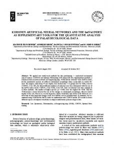
Scope In this fourth and final part of the tutorial review series several miscellaneous aspects required for working with neural networks such as data processing; performance evaluation; generalization and overtraining; some basics in the data structures used in neural networks, namely, vectors and matrix; neural network simulation software; books and internet resources on artificial neural networks are presented though briefly keeping in view the overall purpose of this tutorial review. Data Collection, Analysis and Processing One of the most important components in the success of any neural network solution is the data. The quality, availability, reliability, repeatability, and relevance of the data used to develop and run the system is critical to its success. Data processing starts from the data collection and analysis, followed by pre-processing and then feeds to the neural network. Finally, post-processing is needed to transform the outputs of the network to the required outputs, if necessary. The whole process is illustrated in figure 1. Let us see some of the most important considerations involved in processing data for neural networks. Types of Variables The types of variables have already been discussed in the part-1 of this review in a section titled ‘A Bit of Math!’ It would be emphasized that all inputs to neural networks should be in numerical format. Data Collection The data collection plan typically consists of three tasks: 1. Identifying the data requirement: The first thing

Data Collection & Analysis

to do when planning data collection is to decide what data we need to solve the problem. In general, it will be necessary to obtain the assistance of some experts in the field. We need to know: a) What data are definitely relevant to the problem; b) What data may be relevant; c) What data are collateral. Both relevant and possibly relevant data should be considered as inputs to the application. 2. Identifying data sources: The next step is to decide from where the data will be obtained. This will allow us to make realistic estimates of the difficulty and expense of obtaining it. If the application demands real time data, these estimates should include an allowance for converting analogue data to digital form. In some cases, it may be desirable to obtain data from a simulation of the real situation. This could be the case if the application is intended to monitor conditions which have health, safety or significant cost implications. Care must be taken to ensure that the simulation is accurate and representative of the real case. 3. Determining the data quantity: It is important to make a reasonable estimation of how much data we will need to develop the neural network properly. If too little

Data Pre-Processing

Neural Network

Data Post-Processing

Figure 1: Data flow chart for neural networks Indian J.Pharm. Educ. 39(3) July - Sept. 2005

117

data is collected, it may not reflect the full range of properties that the network should be learning, and this will limit its performance with unseen data. In general, the quantity of data required is governed by the number of training cases that will be needed to ensure the network performs adequately. The intrinsic dimensionality of the data and the required resolution are the main factors determining the number of training cases and, therefore, the quantity of data required. Preliminary Data Analysis There are two basic techniques which can be used to help us understand the data. 1. Statistical analysis: Neural networks can be regarded as extensions of standard statistical techniques, and so such tests can give us an idea of the performance the network is likely to achieve. In addition, analysis can give useful clues to the defining features - for example, if the data is divided into classes, a statistical test can determine the possibility of distinguishing between the different classes in raw data or pre-processed data. 2. Data visualization: Plotting a graph of the data in a suitable format enables us to spot distinguishing features, such as kinks or peaks, which characterize the data. This will enable us to plan and, if practicable, test the pre-processing required to enhance those features. Preliminary data analysis often combines both visualization and statistical tests in an iterative manner. Visualization gives an appraisal of the data, and ideas about the underlying patterns, while statistical analysis enables us to test those ideas. 3. Data Partitioning: Partitioning is the process of dividing the data into validation sets, training sets, and test sets. By definition, validation sets are used to decide the architecture of the network; training sets are used to actually update the weights in a network; test sets are used to examine the final performance of the network. The primary concerns should be to ensure that: a) the training set contains enough data, and suitable data distribution to adequately demonstrate the properties we wish the network to learn; b) there is no unwarranted similarity between data in different data sets. Data Pre-Processing Theoretically, a neural network could be used to map the raw input data directly to required output data. But in practice, it is nearly always beneficial, sometimes critical to apply pre-processing to the input data before they are fed to a network. There are many techniques and considerations relevant to data pre-processing. Preprocessing can vary from simple filtering (as in time-series data), to complex processes for extracting features from image data. Since the choice of pre-processing algorithms depends on the application and the nature of the data, the range of possibilities is vast. However, the aims of 118

pre-processing algorithms are often very similar, namely 1-3: a) Transform the data into a form suited to the network inputs - this can often simplify the processing that the network has to perform and lead to faster development times. Such transformations may include: · Applying a mathematical function (logarithm or square) to an input; · Encoding textual data from a database; · Scaling data so that it has a zero mean and a standard deviation of one; · Taking the Fourier transform of a time-series. b) Select the most relevant data - This may include simple operations such as filtering or taking combinations of inputs to optimize the information content of the data. This is particularly important when the data is noisy or contains irrelevant information. Careful selection of relevant data will make networks easier to develop and improve their performance on noisy data. c) Minimize the number of inputs to the network Reducing the dimensionality of the input data and minimizing the number of inputs to the network can simplify the problem. In some situations - for example in image processing - it is simply impossible to apply all the inputs to the network. In an application to classify cell types from microscope images, each image may contain a quarter of a million pixels: clearly, it would not be feasible to use that many inputs. In this case, the pre-processing might compute some simple parameters such as area and length/height ratio, which would then be used as inputs to the network. This process is called feature extraction.2 Normalization: Normalization involves scaling the rows to a constant total, usually 1 or 100. This is useful if the absolute concentrations of samples cannot easily be controlled. An example might be biological extracts: the precise amount of material might vary unpredictably, but the relative proportions of each chemical can be measured. Normalizing introduces a constraint which is often called closure. The numbers in the multivariate data matrix are proportions and some of the properties have analogy to mixtures. Standardisation: Standardisation is another common method for data scaling and occurs after mean centering: in addition, each variable is also divided by its standard deviation. Standardisation can be important in many real situations. Consider, for example, a case where the concentrations of 30 metabolites are monitored in a series of organisms. Some metabolites might be abundant in all samples, but their variation is not very significant. The change in concentration of the minor compounds might have a significant relationship to the underlying biology. Data Compression The ratio of the number of samples to the number of adjustable parameters in the artificial neural network Indian J.Pharm. Educ. 39(3) July - Sept. 2005

(ANN) should be kept as large as possible. One way of over-determining the problem is to compress input data. In addition to reducing the size of input data, compression allows one to eliminate irrelevant information such as noise or redundancies present in a data matrix. Successful data compression can result in increased training speed, reduction of memory storage, better generalization ability of the model, enhanced robustness with respect to noise in the measurements and simpler model representation. The most often used method for compressing information with ANN is Principal Component Analysis.4 Principal Component Analysis (PCA): When we collect multivariate data it is not uncommon to discover that at least some of the variables are correlated with each other. One implication of these correlations is that there will be some redundancy in the information provided by our variables. In the extreme case of two perfectly

correlated variables (x & y) one of them is redundant since if we know the value of the x variable the value of the y variable has no freedom and vice versa. Principal Components Analysis (PCA) exploits the redundancy in multivariate data, enabling us to pick out patterns (relationships) in the variables and reduce the dimensionality of our data set without a significant loss of information. Assumes that if we have data for a large number of variables (k ), obtained from n cases, there may be a smaller set of derived variables which retain most of the original information in table 1. Weight and height are probably highly correlated and systolic blood pressure (SBP) and heart rate may be related. Imagine 2 new variables, pc1 and pc2, where pc1 is a combination of weight and height while pc2 is a combination of SBP, age and heart rate.

Table 1: Illustrative multivariate data Case

Height (x1)

Weight (x2)

Age (x3)

Systolic Blood Pressure (x4)

Heart rate (x5)

1

175

1225

25

117

56

2 …

156 …

1050 …

31 …

122 …

63 …

n

202

1350

58

154

67

Figure 2: The Hot Air Balloon in 2D Hence, the number of variables could be reduced from 5 to 2 with little loss of information. These new variables, derived from the original variables, are called components. Thus, the main aim of PCA is to reduce dimensionality with a minimum loss of information. This is achieved by projecting the data onto fewer dimensions that are chosen to exploit the relationships between the variables. Projecting data onto fewer dimensions may sound like science fiction but all are familiar with it. The Hot-Air balloon is 3-dimensional, but its photograph is 2-dimensional. In other words its image has been projected onto fewer dimensions. Although represented in fewer dimensions it can still be recognised Indian J.Pharm. Educ. 39(3) July - Sept. 2005

Figure 3: 2D Projection of 3D Doughnut as a hot-air balloon, because the image retains a significant amount of information. The process of projection can be described mathematically, but here we will use a non-mathematical metaphor. Focus a light onto this doughnut suspended in space from two different directions. These lights cast shadows onto two ‘screens’. The nature of the shadow is dependent on the position of the torch. The two shadows are different projections of the same 3-dimensional doughnut onto the two dimensional screens. If you were sitting behind the screen you would only see the shadow. Whether or not you could recognize these shadows as being cast by a doughnut would depend on their 119

orientations. An obvious, but important point is that the doughnut never changes shape even though the projections are quite different. We have seen that objects can be projected onto fewer dimensions. Some projections retain a lot of information about the object while others do not. Now consider two alternative methods of obtaining the projections. We could move the doughnut and keep the torches stationary or keep the doughnut stationary and move the torches. The projections obtained by these alternative methods would be equivalent; the net effect is the same. Remember this when you begin to think about projections of data rather than doughnuts. The mathematical approach of PCA is the second of these alternatives. The data are never moved, instead we move the axes. This is equivalent to moving the torches. PCA decides, which amongst all possible projections, are the best for representing the structure of your data. Projections are chosen so that the maximum amount of information, measured in terms of variability, is retained in the smallest number of dimensions. There is a very large battery of methods for data preprocessing, although the ones described above are the most common. It is possible to combine approaches, for example, first to normalize and then standardize a data set. Weighting of each variable according to any external criterion of importance is sometimes employed. Logarithmic scaling of measurements might be useful if there are large variations in intensities. Selective normalization over part of the variables is sometimes used, it is even possible to divide the measurements into blocks and perform normalization separately on each block. This could be useful if there were several types of measurement, for example, a couple of spectra and one chromatogram, each constituting a single block. Data Post-Processing Post-processing covers any process that is applied to the output of the network. As with pre-processing, it is entirely dependent on the application and may include detecting when a parameter exceeds an acceptable range, or using the output of a network as one input to a rulebased processor. Sometimes it is just the reverse process of data pre-processing. Evaluation of neural networks A human learner’s capabilities can be evaluated in the following ways. How well does the learner perform on the data on which the learner has been trained, i.e., what is the difference between the expected and actual results generated by the learner? How well does the learner perform on new data not used for training the learner? The performance of neural networks can also be evaluated using the same criteria. 120

Quality of Performance:The performance of a neural network is frequently gauged in terms of an error measure. The error measure most often used is the Euclidean Where is d i is the ith element

distance

of the desired output vector and o i is the ith element of the actual network output vector. Several statistics are used for measuring the predictive ability of a model. Prediction Error Sum of Squares is computed as: where d i is the actual value of d for object i and o i is the predicted value o for object i with the model under evaluation, ei is the residual for object i (the difference between the predicted and the actual value) and n is the number of objects. The Mean Squared Error of Prediction (MSEP) is defined as Its square root is called Root Mean Squared Error of Prediction, . All these quantities give the same information. The nature of the problem sometimes dictates the choice of the error measure. In classification problems, in addition to the Euclidean distance, another possible error measure is the fraction of misclassified samples. For clustering problems, it is desirable that the number of clusters should be small, intra-cluster distances should be small and inter-cluster distances should be large. Generalizability: It is not surprising for a system to perform well on the data on which it has been trained. But good generalizability is also necessary, i.e., the system must perform well on new test data distinct from training data. Consider a child memorizing an answer to a question by memory without learning any pattern in it. While the child can answer exactly to the same question, it may fail to do so if the question is an applied one or twisted. The same distinction between learning and memorization is also relevant for neural networks. In network development, therefore, available data is separated into two parts, of which one part is the training data and other part is the test data. It has been observed that excessive training on the training data sometimes decreases performance on the test data. One way to avoid this danger of “overtraining” is by constant evaluation of the system using the test data as learning proceeds. After each small step of learning (in which performance of the network on training data improves), one must examine whether performance on test data also improves. If there is a succession of training steps in which performance improves only for the training data and not for the test data, overtraining is considered to have occurred, and the training process should be terminated. Indian J.Pharm. Educ. 39(3) July - Sept. 2005

Overtraining & Generalizability Given a large network, it is possible that repeated training iterations successively improve performance of the network on training data, e.g., by “memorizing” training samples, but the resulting network may perform poorly on the test data. This phenomenon is called overtraining or over-fitting by the neural network.5, 6 Many important issues, such as determining how many training samples are required for successful learning, and how large a neural network is required for a specific task, are solved in practice by trial and error. These issues are complex because there is considerable dependence on the specific problem being attacked using a neural network.5 With too few nodes, the network may not be powerful enough for a given learning task. With a large number of nodes (and connections), computation is too expensive and also it may essentially “memorize” the input training samples; such a network tends to perform poorly on new test samples, and is not considered to have accomplished learning successfully. Neural learning is considered successful only if the system can perform well on test data on which the system has not been trained. Therefore emphasis is on the capabilities of a network to generalize from input training samples, not to memorize them. 5 One either begins from a large network and successively removes some nodes and links until network performance degrades to an unacceptable level; or begins from a very small network and introduces new nodes and weights until performance is satisfactory; the network is retrained at each intermediate state.5 Based on how the network performs its function, we see that the size of the network (model complexity) is related to performance: Too few degrees of freedom (weights) affect the network’s ability to achieve good fit to the target function. If the network is too large, however, it will not generalize well, because the fit is too specific to the training-set data (memorization). An intermediate network size is our best choice. Therefore, for good performance, methods controlling the network complexity become indispensable in the methodology. The problem of network size can be stated in a simplified manner as follows: Any learning machine should be sufficiently large to solve the problem, but not larger.7 Overtraining and hence over fitting the training data can be avoided if a monitoring set is used to stop the training at an appropriate point. The evolution of the monitoring error must be followed during training. The frequency of monitoring error estimation has to be determined by the user; ideally it should be performed after each iteration. Consecutive monitoring error values are stored in a vector, and several criteria can be applied to retain the optimum set of weights: train the NN for a Indian J.Pharm. Educ. 39(3) July - Sept. 2005

pre-defined large number of iterations and retain the set of weights corresponding to the minimum of the monitoring error curve; stop training and retain the last set of weights as soon as the monitoring error is below a pre-specified threshold or stop training and retain the last set of weights as soon as the decrement between two successive monitoring errors is below a pre-specified threshold.4 Grounding in Vector and Matrix Multivariate data is conveniently handled by matrix notations and manipulations. The concept of matrix as applied to ANN has been discussed in the first part. Let us recall that in a matrix we can treat the rows to represent different examples, (objects) and the columns to represent the variables (properties) of the object, for instance the column could represent the absorbances at different wave lengths of a spectrum where each row refers to a spectrum of different sample (object). N th Axis xn (x 1, x 2, x 3, …,xn ) x2

x1

2nd Axis

1 st Axis

Figure 4: The vector projected as a point in N-dimensional space.

y x

y

Figure 5: Projection of a vector on another.

A single number is often called a scalar and denoted in italics, e.g. x. A vector consists of a row or column of numbers and is denoted as bold lower case italics e.g. x. For example x = [3 5 9 -2] is a row vector and y =

a column vector, these could

be the x, y, z coordinates for a point in 3D space. A 121

vector x can be represented by a directed line segment that has the origin of the space as its initial point and the point with coordinates (x 1, x 2, x 3, …,x n) as its end point as shown in the figure 4. The transpose of a column vector x is denoted either as x’ or as xT, and it is a row vector with the same elements.

 x1    T [x x =  Μ , x = 1  xn 

Λ

xn ] .

X= The transpose of a row

vector produces a column vector. Length (or Norm) of a vector is a function that produces a scalar. The bestknown norm is the L2 norm. The L2 norm of a vector is a scalar that is equal to its length. The norm is denoted by || and is computed as

The inner product of two vectors x = [x 1, x 2, …,x n]T and y = [y1, y2, …,yn]T is the scalar

are normally presented with the number of rows first and the number of columns second, and vectors can be represented as matrices with one dimension equal to 1, so that x above has dimension 1 × 4 and X has dimension 2 × 3 . A square matrix is one where the number of columns equals the number of rows. For example

Y =

is a square matrix. The individual

elements of a matrix are often referenced as scalars, with subscripts referring to the row and column; hence in the matrix above, y21 = 0 which is the element in row 2 and column 1. Transposing a matrix involves swapping the columns and rows around, and is denoted by a righthand-side superscript. For example the transpose of X

The

inner product can be visualized as the projection of one vector onto the other as shown in figure 5. The inner product is a very common operation with vectors. Note that the inner product of a vector with itself gives the square of its length. Another notation for the inner

defined by

is a matrix. The dimensions of a matrix

The

length of a vector in an N-dimensional space is simply the extension of the Pythagorean Theorem to N dimensions, so the L2 norm corresponds to the Euclidean distance. Inner or dot product is the vector operation equivalent to the multiplication of real numbers.

product

because they can be composed from other elements in the set. A linearly independent set of vectors is minimal; we need them all since we cannot represent any as a sum of the others. A matrix is a two dimensional array of numbers and is denoted as bold upper case italics e.g. X. for example

is x·y. The angle between two vectors is Two vectors are orthogonal

when the angle between them is 90 degrees, which implies that their inner product is zero (cos90 = 0). The concept of orthogonality can also be extended to spaces. A vector is orthogonal to a space when it is orthogonal to all vectors in the space; that is the vector must lie along the normal to the space. The vectors that lie along the axes of N-dimensional space are orthogonal. For example it is x, y and z axis for three dimensional space. However, there are other, less obvious combinations that make vectors orthogonal (use the inner product definition). When the norm of the orthogonal vectors is set to 1, the set is called orthonormal. Dividing each orthogonal vector by its length creates the orthonormal set.

denoted X' =

Matrix and vector multiplication

using the ‘dot’ product is denoted by the symbol ‘.’ between matrices. It is only possible to multiply two matrices together if the number of columns of the first matrix equals the number of rows of the second matrix. The number of rows of the product will equal the number of rows in the first matrix, and the number of columns equals the number of columns in the second matrix. Hence a 3 × 2 matrix when multiplied by 2 × 4 matrix will give a 3 × 4 matrix. Multiplication of matrices is not commutative (A.B is not equal to B.A) even if the second product is allowable. Matrix multiplication can be expressed as summations. For arrays with more than two dimensions, it is probably easier to think in terms of summations. If matrix A has dimensions i × j and matrix B has dimensions j × k then the product C of dimensions i × k has elements defined by

Hence

A set of vectors {x i} is called linearly independent if the equation a 1x 1 + a 2x 2 + … +a nx n = 0 is true if and only if all the constants a i are zero. In a linearly dependent set of vectors at least one vector can be represented by a linear combination of the others, so some are superfluous 122

Indian J.Pharm. Educ. 39(3) July - Sept. 2005

Matrix multiplication is distributive and associative. Most square matrices have inverses, defined by the matrix which when multiplied with the original matrix gives the identity matrix, and is represented by a -1 as a right-handside superscript, so that D.D-1 = I. In any square matrix, the elements running diagonally from the top left-hand corner form the leading diagonal. A square matrix in which all the elements in the leading diagonal are equal to 1 and the remainder are equal to zero is called an identity matrix or unit matrix. The unit matrix is the matrix equivalent to unity in classical mathematics, because if a matrix is multiplied by a unit matrix, the answer will be the original matrix. Note that some square matrices do not have inverses: this is caused by there being correlations in the columns or rows of the original matrix. Just as in vectors, the addition / subtraction of two matrices of the same size produces a third matrix of the same size with elements that the addition / subtraction of the elements with the same index. Multiplication of a matrix by a constant equals the multiplication of each element of the matrix by the constant. All the elements of a null matrix are zero. A null matrix is the matrix equivalent of zero in classical mathematics. The product of any matrix with the null matrix of the same order is equal to zero. To gain deeper understanding and enough grounding on the subject, readers are advised to refer any good book8 on linear algebra.

l

STATISTICA Neural Networks is a comprehensive application capable of designing a wide range of neural network architectures, employing both widelyused and highly-specialized training algorithms. Developed by StatSoft, Inc. (www.statsoft.com.), it is available as a stand-alone product or a seamless add-on to STATISTICA – one of the popular statistical software.

l

NeuroSolutions™ from NeuroDimension, Inc., (http:/ /www.nd.com) is a neural network simulation environment with intuitive icon-based graphical user interface. It provides for a wide variety of predesigned network architectures as well as allows the creation of custom network architectures. The software has extensive probing/visualization capabilities. NeuroDimension also markets an Microsoft Excel add-in named NeuroSolutions for Excel that allows you to use Neurosolutions directly from Microsoft Excel.

l

NeuNet Pro is a complete neural network development system. Neural networks can be used for pattern recognition, data mining, market forecasting, and medical diagnosis ... almost any activity where you need to make a prediction based on your data. For information about NeuNet Pro, visit the website at http://www.cormactech.com/neunet

l

OpenAi is a free GUI based neural network simulation software developed in java, Copyright 2001, OpenAi Labs., http://www.openai.net/contact.html.

l

JOONE: Java Object Oriented Neural Engine is free software developed primarily by Paolo Marrone and is available from http://www.joone.org. Joone is a Java framework to build and run Artificial Intelligence applications based on neural networks. Joone applications can be built on a local machine, be trained on a distributed environment and run on whatever device. BrainMaker Neural Network Software is extremely sophisticated neural network software with great documentation, optional accelerator boards. No special programming or computer skills are required. All that is needed is a PC with Windows 2000 or XP and sample data to build your own neural network. It is a product of California Scientific (http:// www.calsci.com).

Neural network simulation software Some of the most popular neural networks simulation software is listed below and several other software packages can be found on the Web by a simple search. l

l

“Stuttgart Neural Network Simulator” from the University of Stuttgart, Germany. A luxurious simulator for many types of nets; with X11 interface: Graphical 2D and 3D topology editor/visualizer, training visualization, etc. Currently supports backpropagation, counter-propagation, generalized radial basis functions (RBF) and many more. Available through anonymous ftp from ftp.informatik.uni-stuttgart.de [129.69.211.2] Directory: /pub/SNNS. A java version JNNS has been made available by the same group. MATLAB Neural Network Toolbox from The Mathworks Inc. (http:// www.mathworks.com ) is a powerful collection of MATLAB functions for the design, training, and simulation of neural networks. It supports a wide range of network architectures with an unlimited number of processing elements and interconnections The Toolbox is delivered as MATLAB M-files, enabling users to see the algorithms and implementations, as well as to make changes or create new functions to address a specific application.

Indian J.Pharm. Educ. 39(3) July - Sept. 2005

l

l

The PDP++ v3.1 software is a neural-network simulation system written in C++. It represents the next generation of the PDP software originally released with the McClelland and Rumelhart “Explorations in Parallel Distributed Processing Handbook”, MIT Press, 1987. It is easy enough for novice users, but very powerful flexible for research use and free to use without commercial motive. It 123

can be freely downloaded from ftp://cnbc.cmu.edu/ pub/pdp++. Books on neural networks A number of books have been authored primarily by the engineering community. Many of such books have been listed in the reference section of each part of the tutorial review. Interested readers who are fascinated by the subject would like to dig deeper into the field of neural networks can refer to any of the following books. The three books authored by L. Fausett; Kishen Mehrotra et al; and Robert J. Schalkoff can make for good starter. l

l

l

l

l

l

l

l

Bishop, C. (1995). Neural Networks for Pattern Recognition. Oxford: University Press. Extremely well-written, up-to-date. Requires a good mathematical background, but rewards careful reading, putting neural networks firmly into a statistical context. Carling, A. (1992). Introducing Neural Networks. Wilmslow, UK: Sigma Press. A relatively gentle introduction. Starting to show its age a little, but still a good starting point. Fausett, L. (1994). Fundamentals of Neural Networks. New York: Prentice Hall. A well-written book, with very detailed worked examples to explain how the algorithms function. Haykin, S. (1994). Neural Networks: A Comprehensive Foundation. New York: Macmillan Publishing. A comprehensive book, with an engineering perspective. Requires a good mathematical background, and contains a great deal of background theory. Ripley, B.D. (1996) Pattern Recognition and Neural Networks. Cambridge University Press. A very good advanced discussion of neural networks, firmly putting them in the wider context of statistical modeling. Rumelhart, D. E. and McClelland, J. L. (1986) Parallel Distributed Processing: Explorations in the Microstructure of Cognition (volumes 1 & 2). The MIT Press. Wasserman, P. D. (1989). Neural Computing: Theory & Practice. Van Nostrand Reinhold: New York. Kohonen, T. (1984) Self-organization and Associative Memory. Springer-Verlag: New York. (2nd Edition: 1988; 3rd edition: 1989).

l

Jure Zupan and Johann Gasteiger, (1999) Neural networks in chemistry and drug design, Wiley-VCH Verlag GmbH, Weomheim,Germany.

l

Devillers, J., (Ed.), (1996) Neural Networks in QSAR and Drug Design, Academic Press, London.

124

Neural network resources on the Internet There exist numerous resources on the Internet to be listed here exhaustively hence only few are listed here. One can find many with the help of any of the popular search engines. Neural Networks Warehouse http://neuralnetworks.ai-depot.com/ Peter Geczy Neural Networks http://www.mns.brain.riken.go.jp/~geczy/Links.html International Neural Network Society http://cns-web.bu.edu/inns/ Sheffield - Neural Networks Course http://www.shef.ac.uk/psychology/gurney/notes/ Neural Networks at your Fingertips http://www.neural-networks-at-your-fingertips.com Usenet groups on NN news://comp.ai.neural-nets/ Neural Network Group http://www.mbfys.kun.nl/Groups/NeuralNetwork Neural Networks Research Centre http://nucleus.hut.fi/nnrc.html Neural Web http://www.erg.abdn.ac.uk/projects/neuralweb/ It is hoped that this four part tutorial review would have given some insights into the field of ANN and illustrated its implications. To conclude, we quote Ralph Waldo Emerson: “Unless you try to do something beyond what you have already mastered, you will never grow”. References 1. Masters, T., Practical Neural Network Recipes in C++. Academic Press, 1993 2.

Bishop, C.M., Neural Networks for Pattern Recognition, Oxford University Press, 1995

3.

Sarles, W.S., Neural Network FAQ, periodic posting to the Usenet newsgroup comp.ai.neural-net, URL: ftp://ftp.sas.com/pub/neural/FAQ.html, 1997

4.

Despagne, F. and Massart, D.L., Analyst, 123, 1998, 157R.

5.

Kishen Mehoratra, Chilukuri K. Mohan, Sanjay Ranka, Elements of Artificial Neural Networks, Massachusetts, USA: The MIT Press, 1997. Schalkoff, R.J., Artificial Neural Networks, New York: McGraw-Hill, 1997.

6. 7.

Jose C. Principe, Neil R. Euliano and W. Curt Lefebvre, Neural and Adaptive Systems: fundamentals through Simulations, New York: John Wiley, 2000.

8.

Nicholson, W.K., Elementary Linear Algebra, with applications, Boston: PWS-Kent Publishing Company, 1990.

Indian J.Pharm. Educ. 39(3) July - Sept. 2005