a variety of other instance-based ensemble pruning approaches in a variety of .... cast as a multi-label classification task: Learning to predict the subset of ...
Instance-Based Ensemble Pruning via Multi-Label Classification Fotini Markatopoulou, Grigorios Tsoumakas and Ioannis Vlahavas Department of Informatics Aristotle University of Thessaloniki Thessaloniki, Greece 54124 Email: {fmarkato,greg,vlahavas}@csd.auth.gr Abstract—Ensemble pruning is concerned with the reduction of the size of an ensemble prior to its combination. Its purpose is to reduce the space and time complexity of the ensemble and/or to increase the ensemble’s accuracy. This paper focuses on instancebased approaches to ensemble pruning, where a different subset of the ensemble may be used for each different unclassified instance. We propose modeling this task as a multi-label learning problem, in order to take advantage of the recent advances in this area for the construction of effective ensemble pruning approaches. Results comparing the proposed framework against a variety of other instance-based ensemble pruning approaches in a variety of datasets using a heterogeneous ensemble of 200 classifiers, show that it leads to improved accuracy.
I. I NTRODUCTION Ensemble methods [1] has been a very popular research topic during the last decade. Their success arises largely from the fact that they offer an appealing solution to several interesting learning problems of the past and the present, such as improving prediction accuracy, scaling inductive algorithms to large databases, learning from multiple physically distributed data sets and learning from concept-drifting data streams. One dimension along which we could categorize ensemble methods is based on the number of models that affect the final decision. Usually all models are taken into consideration. When models are classifiers, this is called classifier fusion. Some methods, however, select just one model from the ensemble. When models are classifiers, this is called classifier selection. A third option, standing in between of these two, is to select a subset of the ensemble’s models. This is mainly called ensemble pruning or ensemble selection [2]. Ensemble pruning is more flexible compared to the other two approaches and usually leads to improved accuracy. A large heterogeneous ensemble may consist of both high and low predictive performance models. The latter may negatively affect the overall performance of the ensemble. Pruning these models while maintaining a high diversity among the remaining members of the ensemble improves predictive performance compared to the full ensemble, as well as compared to just a single classifier, which lacks the error-correction mechanism of multiple models. Ensemble pruning is also useful in terms of efficiency. Having a very large number of models in an ensemble adds a lot of computational overhead. For example, decision tree models may have large memory requirements [3] and lazy
learning methods have a considerable computational cost during execution. The minimization of run-time overhead is crucial in certain applications, such as in stream mining. In addition, when models are distributed over a network, the reduction of models leads to the reduction of the important cost of communication. Ensemble pruning methods can be either static, meaning that they select a fixed subset of the original ensemble for all test instances, or dynamic, also called instance-based, where a different subset of the original ensemble may be selected for each different test instance. The rationale of using instance-based ensemble pruning approaches is that different models have different areas of expertise in the instance space. Therefore, static approaches that are forced to select a fixed subset prior to seeing an unclassified instance may have a theoretical disadvantage compared to dynamic ones. This paper proposes a new approach to the instance-based ensemble pruning problem by modeling it as a multi-label learning task [4]. Labels correspond to classifiers and multilabel training examples are formed based on the ability of each classifier to correctly classify each original training example. This way we can take advantage of recent advances in the area of multi-label learning and attack collectively, instead of separately, the problems of predicting whether each classifier will classify correctly a given unclassified instance. The rest of this paper is organized as follows. Section 2 reviews related work on instance-based ensemble pruning. Section 3 presents the proposed approach, Section 4 the empirical study and Section 5 the conclusions. II. I NSTANCE -BASED E NSEMBLE P RUNING Before we start with the presentation of specific instancebased ensemble pruning methods, it is important to clarify two general issues with respect to the space and time complexity respectively. The first one is that contrary to static ensemble pruning methods, which pre-select one specific subset of the original ensemble for all unclassified instances, instance-based ensemble pruning methods cannot really offer any benefit in terms of space complexity, as they need to retain the complete ensemble. The second one is that since the output of these methods depends on just a subset of the models of the original
ensemble, one would expect that there are always gains in terms of time complexity. However, this is not necessarily true. Some methods (e.g. LCA variant in [5]) first query all models and then select a subset of those to combine. Others might require computations that are more expensive compared to querying all models. For example, locating the 10 nearest neighbors of a new unclassified instance and then querying one decision tree, might be more expensive compared to directly querying 100 decision trees. Therefore, only computationally simple approaches to pruning, such as [6] can guarantee improved time complexity in the general case, sometimes at the expense of accuracy. The primary goal of most of the other methods is improving the accuracy compared to the complete ensemble. The proposed approach falls into this latter category of methods. It aims at improved accuracy and cannot guarantee time complexity improvements as it first needs to query a multi-label learner. Few approaches deal directly with instance-based ensemble pruning [7], [8], [9], [6]. These are presented in subsection II-B. However, there are also some that deal with dynamic approaches to classifier selection and fusion [5], [10], [11], [12], which can be considered as extreme cases of ensemble pruning. In addition, some dynamic classifier selection approaches, may in some cases (e.g. ties) take into consideration more than one model. We therefore discuss here such methods too (subsection II-A). We close the section with a discussion on instance-based ensemble pruning and diversity (subsection II-C). A. Dynamic Classifier Selection and Fusion The approach in [5] starts with retrieving the 𝑘 nearest neighbors of a given test instance from the training set. It then classifies this test instance using the most competent classifier within this local region. In case of ties, majority voting is applied. The local performance of classifiers is assessed using two different metrics. The first one, called overall local accuracy (OLA), measures the percentage of correct classifications of a model for the examples that exist in the local region. The second one, called local class accuracy (LCA), measures the percentage of correct classifications of a model within the local region too, but only for those examples where the model had given the same output as the one it gives for the current unlabeled instance being considered. A very similar approach to this one was proposed independently at the same time [10], also taking the distance of the 𝑘 nearest neighbors into account. The dynamic selection (DS) and dynamic voting (DV) approaches in [11], [13] are in the same spirit as [5], [10]. A 𝑘NN approach is initially used to find the most similar training instances with the given test instance. DS selects the classifier with the least error within the local area of the neighbors weighted by distance. In fact, DS, is very similar to the weighted version of OLA presented in [10]. DV is different, as it is a classifier fusion approach. It combines all models weighted by their local competence.
Yet another approach along the same lines is [14]. After finding the 𝑘 nearest neighbors of the test instance, this approach further filters the neighborhood based on the similarity of the predictions of all models for this instance and each neighbor. In this sense, this approach is similar to the LCA variation in [5]. It finally selects the most competent classifier in the reduced neighborhood. The predictions of all models for an instance, are in this paper called collectively multiple classifier behavior (MCB). The approach in [12] estimates whether the ensemble’s models will be correct /incorrect with respect to a given test instance, using a learning algorithm, trained from the 𝑘-fold cross-validation performance of the models on the training set. It can be considered as a generalization of the approaches we have seen so far in this subsection, where a nearest neighbor approach was specifically used instead. The approach we propose in this paper, is based on the same principle, with the difference that multi-label learning algorithms are employed and therefore the binary tasks of predicting correct/incorrect decision for each model are viewed in a collective way. B. Dynamic Ensemble Selection Dynamic Voting with Selection (DVS) [7], [15] is an approach that stands in between the DS and DV algorithms that were mentioned in the previous subsection. First, about half of the models in the ensemble, those with local errors that fall into the upper half of the error range of the committee, are discarded. Then, the rest are combined using DV. Since this variation, eventually selects a subset of the original models, we can consider it as an instance-based ensemble pruning approach. The primary goal of 𝑘-nearest-oracles (KNORA) [9] is improving the accuracy compared to the complete ensemble. Four different versions of the basic KNORA algorithm are proposed, all based on an initial stage of identifying the 𝑘 nearest neighbors of a given unclassified instance. KNORAELIMINATE selects those classifiers that correctly classify all 𝑘 neighbors. In case none such exists, the 𝑘 value is decreased until at least one is found. KNORA-UNION selects those classifiers that correctly classify at least one of the 𝑘 neighbors. KNORA-ELIMINATE-W and KNORA-UNION-W are variations that weight the votes of classifiers according to their Euclidean distance to the unclassified instance. Recently, a statistical approach has been proposed for instance-based pruning of homogeneous ensembles, with the provided that the models are produced via independent applications of a randomized learning algorithm on the same training data, and that majority voting is used [6]. It is based on the observation that given the decisions made by the classifiers that have already been queried, the probability distribution of the remaining class predictions can be calculated via a Polya urn model. During prediction, it samples the ensemble members randomly without replacement, stopping when the probability that the predicted class will change is below a specified level. As this approach assumes homogeneous models, it aims at speeding up the classification process
without significant loss in accuracy. In contrast, our approach is directed at heterogeneous ensembles and aims primarily at improving the predictive performance compared to the full ensemble. Another approach with the same goal as [6] is [8]. In that work a first stage of static pruning takes place, followed up by a second stage of dynamic pruning, called dynamic scheduling. In the dynamic stage, classifiers are considered one by one in a decreasing order of total benefit (the authors focused on costsensitive applications). This iterative process stops when the difference of the current ensemble and the complete ensemble, as estimated assuming normal distribution with parameters calculated on the training set, is small. C. Instance-Based Ensemble Pruning and Diversity A potential point of criticism against most of the presented dynamic classifier combination methods, as well as against the proposed framework, could be that they are focused on accuracy and ignore diversity. The question is, should diversity be a desired property of the ensembles selected by instancebased ensemble pruning methods? The concept of diversity has been studied extensively [16] and it is generally accepted that diversity and accuracy are both required for a successful ensemble. Diversity is desired, because models that err in different parts of the input space can help each other correct their mistakes through a voting process. In instance-based approaches however, we are interested in the performance for a specific example, not the whole input space in general, or a part of it. In this case we would want to choose only those models that are as accurate as possible for this example, and not those models that may make mistakes in it. Our approach is based solely on accuracy to select the appropriate subset of the ensemble. Note, however, that diversity is still crucial as a property of the full ensemble. III. T HE P ROPOSED F RAMEWORK : IBEP-MLC Let (𝑥⃗𝑖 , 𝑦𝑖 ), 𝑖 = 1 . . . 𝑛, denote a set of 𝑛 training examples, where each input vector 𝑥⃗𝑖 consists of 𝑚 values 𝑥𝑖1 , . . . 𝑥𝑖𝑚 , while 𝑦𝑖 is the value of the target variable. From this training set we construct an ensemble of 𝑇 classifiers 𝐶1 , . . . , 𝐶𝑇 , using the ensemble construction technique of our choice. Let 𝐶𝑗 (𝑥⃗′ ) denote the prediction of classifier 𝐶𝑗 for a test input vector The proposed framework is based on the simple observation that the problem of instance-based ensemble pruning can be cast as a multi-label classification task: Learning to predict the subset of classifiers that are expected to correctly classify a given instance. We dub this framework Instance-Based Ensemble Pruning via Multi-label Classification (IBEP-MLC). The framework requires the construction of an appropriate multi-label training set for this learning task. The feature space of this training set is the same as the original feature space, while the label space contains one label for each classifier. Multi-label training examples can be constructed by querying each classifier in the ensemble with training instances, 𝑥⃗𝑖 , and
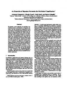
comparing their output with their true output, 𝑦𝑖 . If the classifiers are produced by different learning algorithms or different parameters of the same learning algorithm, then 𝑘-fold crossvalidation can be used to obtain unbiased predictions. If the prediction of a classifier is correct then a positive class value is used for the corresponding label, while if the prediction is incorrect then a negative class value is used. Figure 1 exemplifies this process for the image segmentation dataset (segment) of the European project Statlog [17]. The target attribute of this dataset has 6 values: brickface, sky, foliage, cement, window, path, grass. Having constructed this training set, what remains is to train a multi-label learner. An interesting question here, is what should be the properties of the multi-label learning algorithm selected for this task and/or what should be an appropriate loss function for training it. We will come back to these questions, after examining first, how the framework predicts the class for an unlabeled instance. Given an unlabeled instance, the multi-label classifier is first queried, outputting a subset of models that it considers that they will classify correctly this instance. Then, each of the models in the subset are queried and their decisions are combined via simple majority voting, also called plurality voting. Let’s denote the subset of classifiers output by the multilabel learner as 𝑍 and the classifiers that are actually correct as 𝑌 . Assuming a two-class problem, the final prediction will be correct if more than half of the models in 𝑍 are correct, or in other words if ∣𝑍 ∩ 𝑌 ∣/∣𝑍∣ > 0.5. This is actually the definition of the precision of a multi-label prediction [18], [4]. For problems with more than two class values, a precision value lower than 0.5, could in some cases also suffice for a correct final decision through plurality voting. The conclusion is that learning algorithms that optimize precision should be used in this task. A zero-one loss function can be defined as follows: { 𝑙𝑜𝑠𝑠(𝑍, 𝑌 ) =
0 if ∣𝑍 ∩ 𝑌 ∣/∣𝑍∣ > 0.5 1 otherwise
(1)
A loss function based on precision could also be defined. However, in this case, the problem is how to penalize the learner for outputting the empty set. A relevant important issue to note, is that some multilabel learning algorithms just output a score vector for each label [19], [20], so they cannot be used without modifications in our case, where a bipartition of the labels into relevant and irrelevant is required. In addition, several of the stateof-the-art multi-label classification algorithms (i.e those that output a bipartition) of the recent literature [21], [22], [23], [24], actually output a score vector primarily and employ a thresholding method [25], [26], [27], [28] in order to be able to output bipartitions. Given that high precision is crucial for the success of IBEP-MLC, we could use the above algorithms in conjunction with a thresholding method that optimizes precision.
Fig. 1.
training set ⃗𝑥 𝑦 𝑥⃗1 sky window 𝑥⃗2 𝑥⃗𝑛
𝐶1 path sky
... foliage
Creating the multi-label training set
classifier predictions 𝐶2 ... sky ... window ...
𝐶𝑇 cement window
foliage
grass
...
path
∙
We experimented on 21 data sets from the UCI Machine Learning repository [29]. Table I presents the details of these data sets (Folder in UCI server, number of instances, classes, continuous and discrete attributes, percentage of missing values). We avoided using datasets with a very small number of examples, so that an adequate amount of data is available for training, testing and meta-data creation via 𝑘-fold crossvalidation.
∙
TABLE I D ETAILS OF DATA SETS : F OLDER IN UCI SERVER , NUMBER OF INSTANCES , CLASSES , CONTINUOUS AND DISCRETE ATTRIBUTES ,
∙
A. Datasets
PERCENTAGE OF MISSING VALUES
id
multi-label training set 𝐶1 𝐶2 ... − + ... − + ...
𝐶𝑇 − +
𝑥⃗𝑛
... −
−
...
IV. E XPERIMENTAL S ETUP
d1 d2 d3 d4 d5 d6 d7 d8 d9 d10 d11 d12 d13 d14 d15 d16 d17 d18 d19 d20 d21
⇒
⃗𝑥 𝑥⃗1 𝑥⃗2
UCI Folder anneal balance-scale breast-w car cmc colic credit-g dermatology ecoli haberman heart-h heart-statlog hill hypothyroid ionosphere kr-vs-kp primary-tumor segment sick sonar soybean
Inst
Cls
Cnt
Dsc
MV(%)
798 625 699 1728 1473 368 1000 366 336 306 294 270 607 3772 351 3196 339 2310 3772 195 683
6 3 2 4 3 2 2 6 8 2 5 2 2 4 2 2 2 7 2 2 19
9 4 0 0 2 7 7 1 7 3 6 13 100 7 34 0 0 19 7 60 0
29 0 2 6 7 15 13 33 0 0 7 0 0 30 0 36 17 0 23 0 35
0.00 0.00 0.00 0.00 0.00 23.80 0.00 0.00 0.00 0.00 20.46 0.00 0.00 5.4 0.00 0.00 0.00 0.00 5.40 0.00 0.00
B. Ensemble Construction We constructed a heterogeneous ensemble of 200 models, by using different learning algorithms with different parameters on the training set. The WEKA machine learning library [30] was used as the source of learning algorithms. We trained 40 multilayer perceptrons (MLPs), 60 𝑘 Nearest Neighbors (𝑘NNs), 80 support vector machines (SVMs) and 20 decision trees (DT) using the C4.5 algorithm. The different parameters used to train the algorithms were the following (default values were used for the rest of the parameters):
∙
+
...
MLPs: we used 5 values for the nodes in the hidden layer {1, 2, 4, 8, 16}, 4 values for the momentum term {0.0, 0.2, 0.5, 0.9} and 2 values for the learning rate {0.3, 0.6}. 𝑘NNs: we used 20 values for 𝑘 distributed evenly between 1 and the plurality of the training instances. We also used 3 weighting methods: no-weighting, inverseweighting and similarity-weighting. SVMs: we used 8 values for the complexity parameter {10−5 , 10−4 , 10−3 , 10−2 , 0.1, 1, 10, 100}, and 10 different kernels. We used 2 polynomial kernels (of degree 2 and 3) and 8 radial kernels (gamma ∈ {0.001, 0.005, 0.01, 0.05, 0.1, 0.5, 1, 2}). Decision trees: We constructed 10 trees using postpruning with 5 values for the confidence factor {0.1, 0.2, 0.3, 0.5 } and 2 values for Laplace smoothing {true, false}, 8 trees using reduced error pruning with 4 values for the number of folds {2, 3, 4, 5} and 2 values for Laplace smoothing {true, false}, and 2 unpruned trees using 2 values for the minimum objects per leaf {2, 3}.
C. Instance-Based Ensemble Pruning Methods We compare the proposed framework against all of the methods that were presented in section 2 and deal with the issue of accuracy improvement. We here describe how these methods were configured. Methods OLA, LCA, MCB, DV, DS, DVS and KNORA start by finding the 𝑘 nearest neighbors of a test instance in the training set. The number of neighbors is set to 10 for all these methods. Euclidean distance is used as distance function to estimate the nearest neighbors. The ELIMINATE version of KNORA was used, as that was found as producing the overall best results in [9]. We also calculate the performance of the complete ensemble of 200 models using simple majority voting for model combination (MV) as a baseline method. We instantiate the proposed framework with two multi-label learning algorithms. The first one is ML-𝑘NN [31], which was selected because it follows an instance-based approach, similarly to the rest of the competing methods, apart from MV. The number of neighbors is also set to 10 here, which happens to be the default setting too. The second one is Calibrated Label Ranking (CLR) [32], a recent high performance multilabel learner that is known to achieve high precision. The C4.5 learning algorithm is used for the binary classification tasks considered by CLR.
D. Evaluation Methodology We use 10-fold cross validation to evaluate the different instance-based pruning approaches. For each of the 10 train/test splits, we perform an inner 10-fold cross-validation on the training set in order to gather meta-data concerning the performance of the algorithms, which are required by all instance-based pruning approaches. V. E XPERIMENTS A. Thresholding the Multi-Label Learners Given that high precision is crucial for IBEP-MLC, we here investigate how thresholding affects the accuracy of the framework. We use a simple thresholding strategy that considers a label as positive if its score is higher than a single threshold 𝑡 used for all labels. We explore threshold values ranging from 0.5 to 0.9 with a step of 0.05. Tables II and III show the accuracy percentage of the framework, instantiated with CLR and ML-𝑘NN respectively, for all datasets and all investigated threshold values. The last row shows the average rank of the performance of the different threshold values. We discuss the results in terms of the average ranks, as recommended in [33]. We basically notice that higher thresholds almost monotonically increase the overall performance of the framework. Two exceptions to this rule are in values 0.7 for CLR and 0.9 for ML-𝑘NN. A threshold of 0.9 leads to the best overall result for CLR, while a threshold of 0.85 for ML𝑘NN. In the rest of the experiments we fix the thresholds to these overall best values for all datasets. One could argue that this is unfair, because we tune a parameter by peeking at the test sets. However, we don’t use the best threshold for each dataset, rather a fixed value, which could be suboptimal for some datasets. In our future work we will investigate automatically tuning the threshold for precision optimization as in [34], [23] or explore alternative thresholding strategies, such as RCut and SCut [25]. The outcome of that work may show that even better results can be achieved this way, since the threshold will be separately tuned for each dataset. B. Accuracy Table IV shows the accuracy percentage and average rank of the competing methods in all datasets. We start the analysis of the results based on the average ranks, as suggested in [33], similarly to the previous section. We notice that the best overall results are achieved by the IBEP-MLC using CLR. This is in accordance with our prior knowledge that CLR is an algorithm that achieves good precision performance. On the other hand, using ML-𝑘NN led to slightly worse results and an overall rank of 4.7. The same performance was achieved by KNORA and MCB, while close to this was also DS. Interestingly OLA was overall better than these approaches, with an average rank of 4.3. DV and DVS did not perform that well, while the worst results were that of the static classifier fusion approach of majority voting. We also comment the results in terms of the wins, ties and loses for each pair of algorithms, which are shown in Table
V. We refrain from reporting only the statistically significant wins and loses, following the recommendation in [33]. We notice again the high performance of CLR, which loses in 4 datasets maximum (less than 20% of all datasets) from any method. This time the main competitor seems to be the recently proposed instance-based ensemble selection approach, KNORA. We also performed the Wilcoxon signed ranks test between CLR and its two main competitors, according to the previous analysis, namely OLA and KNORA. In both cases the 𝑝 level was less than 0.01, thus we accept that CLR is overall significantly better with 99% confidence. This result should be taken with slight cautiousness, due to the fact that we did two tests instead of one, and we did not correct for chance effects. Still, 99% is a very strong confidence. C. Number of Selected Models Table VI shows the average number of models selected by dynamic ensemble selection methods IBEP-MLC (with CLR and ML-𝑘NN), KNORA and DVS across all test instances for all datasets. It is clear that one of the reasons for CLR’s success is the selection of a small number of accurate models. ML𝑘NN on the other hand exhibits a strange behavior, sometimes outputting a very small number of models (even just one), while other times a quite large one. This, could be due to the fact that its probability estimates for each label are not as smooth as CLR’s which are calculated based on the average votes of the pairwise binary classifiers. The average number of models selected by both ML-𝑘NN and KNORA is about 100, while that of DVS is even larger, justifying its respective lower performance. TABLE VI AVERAGE NUMBER OF MODELS QUERIED BY DYNAMIC ENSEMBLE SELECTION METHODS . dataset id
DVS
ML-𝑘NN
CLR
KNORA
d1 d2 d3 d4 d5 d6 d7 d8 d9 d10 d11 d12 d13 d14 d15 d16 d17 d18 d19 d20 d21
172±6 131±7 176±10 137±9 94±10 167±6 112±5 134±4 120±44 134±19 141±13 145±8 99±5 141±5 156±17 102±5 89±6 131±2 177±3 111±11 79±11
166±6 86±8 167±16 132±8 1±0 100±11 47±14 127±9 83±73 31±24 98±29 82±20 3±0 182±6 132±26 88±16 4±3 116±2 184±1 22±13 17±9
16±1 19±1 9±2 15±2 12±1 8±2 5±0 18±2 12±5 15±2 10±3 3±1 13±2 20±0 12±1 14±2 11±1 12±1 16±3 3±1 17±2
153±6 51±9 159±19 43±15 56±10 91±14 57±6 103±10 134±54 141±20 114±22 96±13 25±11 139±5 129±29 48±12 78±12 107±3 173±3 50±27 109±34
mean
131±28
89±59
12±5
98±43
TABLE II P ERCENTAGE OF ACCURACY AND AVERAGE RANK OF IBEP-MLC USING CLR AND A THRESHOLD RANGING FROM 0.5 TO 0.9 WITH A STEP OF 0.05 FOR ALL DATASETS . id
0.50
0.55
0.60
0.65
0.70
0.75
0.80
0.85
0.90
d1 d2 d3 d4 d5 d6 d7 d8 d9 d10 d11 d12 d13 d14 d15 d16 d17 d18 d19 d20 d21
98.89±01.05% 88.97±03.26% 96.57±03.88% 83.90±08.96% 26.56±23.07% 84.53±06.10% 75.00±04.81% 97.00±01.99% 65.04±35.43% 72.89±09.47% 80.44±17.49% 83.33±04.70% 55.28±03.16% 93.96±01.42% 89.78±08.86% 93.83±06.35% 44.81±06.75% 96.23±01.89% 97.14±00.92% 46.74±16.80% 84.30±11.35%
99.22±00.75% 88.81±03.41% 96.29±03.94% 84.77±09.23% 27.38±23.20% 83.99±07.12% 74.70±04.95% 97.28±02.21% 65.94±33.71% 72.89±09.47% 80.44±17.49% 83.33±04.70% 55.12±02.77% 94.09±01.34% 89.49±08.64% 94.27±06.13% 45.99±06.79% 96.71±01.97% 97.38±00.93% 47.21±15.50% 86.50±10.30%
99.22±00.75% 88.97±03.44% 96.29±03.94% 84.89±09.63% 28.19±23.07% 83.43±06.91% 75.00±05.72% 97.55±02.00% 67.76±31.92% 72.56±09.25% 80.78±17.50% 83.33±04.00% 56.44±02.56% 94.27±01.37% 90.34±07.68% 94.68±05.88% 46.87±06.52% 96.97±01.77% 97.59±00.84% 47.69±15.74% 87.38±09.53%
99.33±00.78% 89.29±03.72% 96.29±03.94% 84.66±09.81% 29.28±22.92% 83.69±06.77% 75.30±05.91% 97.56±02.00% 68.37±30.57% 73.23±09.42% 81.13±18.24% 83.33±03.60% 56.94±02.67% 94.75±01.46% 90.63±07.66% 95.12±05.46% 47.48±05.12% 97.36±01.76% 97.83±00.76% 47.74±16.83% 88.26±09.06%
99.33±00.78% 89.93±04.02% 96.28±03.88% 85.35±09.32% 29.82±22.12% 83.69±06.02% 75.20±05.71% 97.56±02.00% 69.88±28.87% 72.24±09.11% 80.78±19.02% 82.59±04.95% 58.01±04.25% 95.94±01.15% 91.48±07.77% 95.65±04.75% 46.86±06.18% 97.40±01.72% 98.07±00.74% 49.71±17.33% 89.58±08.86%
99.56±00.78% 91.06±04.42% 96.14±03.81% 86.51±08.92% 30.98±21.56% 84.23±06.52% 75.10±05.65% 97.56±02.00% 68.07±30.01% 72.25±08.83% 80.44±18.87% 82.59±04.95% 59.49±04.36% 97.99±00.71% 91.76±06.73% 95.90±04.62% 46.27±05.97% 97.62±01.46% 98.30±00.83% 50.62±16.18% 89.29±09.07%
99.33±00.78% 93.78±04.82% 96.28±03.88% 87.50±08.95% 30.91±21.42% 83.68±07.39% 75.90±05.90% 97.56±02.00% 67.18±30.08% 71.61±08.63% 81.13±17.65% 82.22±04.88% 60.73±03.93% 99.47±00.18% 92.33±06.80% 96.09±04.01% 46.57±06.39% 97.53±01.31% 98.60±00.64% 50.60±17.14% 89.58±09.68%
99.11±00.70% 96.33±03.27% 96.28±03.88% 88.08±08.54% 31.86±20.15% 84.76±06.11% 74.90±06.23% 97.55±02.00% 68.07±30.01% 71.28±08.49% 82.16±18.20% 82.59±04.95% 61.96±04.63% 99.42±00.33% 93.17±05.22% 95.96±04.27% 47.47±05.24% 97.40±01.40% 98.73±00.75% 53.48±15.12% 89.73±09.47%
99.22±00.75% 97.13±03.33% 96.57±03.70% 88.60±07.36% 32.75±20.18% 83.67±07.28% 75.30±05.50% 98.10±01.83% 69.28±28.80% 71.94±09.79% 81.82±16.71% 80.00±04.68% 63.37±04.36% 99.42±00.33% 94.60±04.54% 95.90±04.37% 47.16±06.99% 97.71±01.46% 98.75±00.59% 55.88±13.31% 89.87±10.17%
Rank
7.4
7.1
6.2
4.6
4.7
4.4
4.1
3.7
2.7
TABLE III ACCURACY AND AVERAGE RANK OF IBEP-MLC USING ML-𝑘NN AND A THRESHOLD RANGING FROM 0.5 TO 0.9 WITH A STEP OF 0.05 FOR ALL DATASETS . id
0.50
0.55
0.60
0.65
0.70
0.75
0.80
0.85
0.90
d1 d2 d3 d4 d5 d6 d7 d8 d9 d10 d11 d12 d13 d14 d15 d16 d17 d18 d19 d20 d21
97.22±01.41% 88.17±03.94% 96.57±04.22% 87.38±07.61% 32.28±16.16% 83.42±05.93% 74.60±05.34% 96.73±01.73% 66.24±34.32% 72.90±09.69% 80.79±15.41% 82.59±03.51% 54.29±02.61% 93.61±01.51% 88.07±09.30% 83.33±17.80% 44.54±05.38% 96.67±01.90% 96.21±01.14% 47.67±18.00% 81.70±10.82%
97.89±01.22% 88.17±03.56% 96.43±04.27% 88.07±08.00% 32.76±15.63% 83.69±06.14% 75.50±05.50% 97.00±01.53% 65.04±35.11% 72.58±08.80% 81.15±15.76% 82.59±03.51% 57.93±06.07% 93.69±01.41% 88.64±09.01% 84.39±17.04% 45.41±05.94% 96.80±01.75% 96.42±01.08% 47.21±18.60% 80.67±11.31%
98.00±01.15% 88.17±03.56% 96.43±04.27% 87.78±07.52% 33.23±15.67% 83.69±06.27% 75.60±04.95% 97.00±01.53% 65.04±35.11% 72.58±07.82% 80.46±15.49% 82.59±03.51% 61.15±06.13% 93.72±01.42% 89.50±08.81% 85.52±15.54% 44.82±06.04% 97.06±01.66% 96.63±01.29% 47.24±18.80% 80.52±11.36%
98.33±00.78% 88.17±03.56% 96.57±03.88% 88.65±06.98% 33.57±15.76% 83.70±06.24% 75.70±03.97% 97.00±01.53% 65.34±35.07% 71.94±09.28% 81.15±15.16% 82.59±03.51% 62.54±05.27% 93.93±01.53% 89.79±08.07% 86.36±14.87% 44.82±06.04% 96.80±01.67% 96.71±01.20% 47.21±16.84% 81.11±11.02%
98.44±00.94% 88.33±03.78% 96.57±03.88% 88.77±06.89% 32.89±15.22% 83.42±06.58% 74.60±04.55% 97.00±01.53% 65.34±34.87% 72.25±08.15% 81.15±14.54% 82.22±03.83% 63.86±06.59% 94.01±01.49% 89.79±08.07% 86.55±14.88% 43.92±07.23% 96.88±01.60% 96.93±01.16% 50.57±16.10% 81.55±10.64%
98.66±01.02% 89.13±03.91% 96.43±03.82% 89.00±07.12% 32.55±15.25% 84.26±06.31% 75.30±03.89% 97.27±01.80% 65.66±33.62% 71.95±08.87% 80.13±15.64% 82.59±03.92% 64.43±06.01% 94.14±01.44% 90.07±07.84% 86.80±15.11% 43.33±06.63% 97.06±01.47% 97.32±01.22% 50.10±15.80% 81.70±10.25%
99.00±01.11% 91.86±04.63% 96.14±04.62% 88.54±07.51% 32.69±15.20% 83.98±06.01% 73.70±05.56% 97.27±01.80% 65.65±34.62% 71.28±09.61% 80.46±16.40% 82.22±04.20% 64.76±06.32% 94.41±01.50% 89.50±08.28% 88.18±12.45% 43.03±07.05% 97.23±01.54% 97.69±00.90% 48.19±16.31% 81.56±10.48%
98.89±01.39% 93.93±04.47% 95.86±04.49% 88.42±07.07% 32.76±15.14% 84.24±06.75% 73.30±05.27% 97.55±02.37% 66.25±34.22% 69.97±10.70% 79.77±15.10% 82.96±03.98% 65.09±06.03% 94.80±01.69% 90.34±08.68% 89.21±11.23% 43.32±06.89% 97.58±01.34% 97.77±00.90% 48.64±16.58% 81.85±10.61%
99.33±00.78% 96.01±02.92% 95.71±03.81% 88.88±06.94% 32.76±15.14% 83.42±07.09% 72.50±05.46% 98.10±02.23% 65.95±33.91% 69.96±11.05% 80.11±14.95% 80.00±05.84% 65.09±05.56% 95.79±01.33% 91.47±07.71% 89.96±11.21% 43.32±06.89% 97.71±01.19% 97.96±00.85% 51.07±14.36% 80.53±09.65%
Rank
6.5
6.1
5.8
4.9
4.8
4.1
4.9
3.8
4.2
VI. C ONCLUSIONS This paper presented a new framework for instance-based ensemble pruning based on multi-label learning. We have shown theoretically, that in order to achieve a correct prediction after a plurality voting process among the subset of models output by the multi-label model, high precision is required. We instantiated this framework with two multilabel learning algorithms and investigated the use of simple
thresholding to improve the precision of the models. We also compared the performance of the proposed framework with its direct competitors and reached to the conclusion that it leads to much better results. Our future worked is planned as follows. Firstly, we want to extend the experimental setup with many more datasets. Secondly, we want to investigate whether thresholding strategies that automatically produce the bipartition from a score vector
TABLE IV P ERCENTAGE OF ACCURACY AND AVERAGE RANK OF THE COMPETING APPROACHES FOR ALL DATASETS . id
MV
OLA
LCA
MCB
DS
DV
DVS
KNORA
ML-𝑘NN
CLR
d1 d2 d3 d4 d5 d6 d7 d8 d9 d10 d11 d12 d13 d14 d15 d16 d17 d18 d19 d20 d21
91.10±02.55% 86.25±03.93% 95.14±06.03% 70.01±13.59% 13.50±10.68% 82.87±05.78% 70.00±04.90% 93.15±05.68% 56.00±44.15% 73.55±09.98% 80.09±19.06% 82.96±03.12% 53.06±03.75% 92.29±01.50% 78.37±16.03% 68.90±21.22% 28.58±08.13% 91.73±03.14% 93.88±01.02% 35.14±20.00% 25.91±20.18%
99.11±01.15% 92.33±05.23% 96.14±03.57% 89.46±07.42% 31.26±18.23% 83.14±07.39% 74.20±04.92% 95.92±02.63% 64.15±34.97% 71.59±07.99% 80.83±13.01% 83.70±03.98% 62.54±04.25% 96.39±01.54% 89.50±08.17% 95.59±04.73% 41.88±06.26% 97.36±01.23% 98.12±00.74% 54.45±14.45% 76.55±17.15%
97.78±01.28% 91.05±01.98% 96.43±04.22% 83.32±09.29% 31.87±20.37% 83.42±05.50% 74.60±04.40% 92.61±05.03% 61.76±37.01% 72.25±08.43% 80.49±12.54% 81.48±04.62% 60.15±04.05% 96.10±01.70% 88.36±08.96% 93.02±06.86% 40.12±05.72% 97.19±01.28% 97.83±00.76% 48.24±20.23% 46.90±18.01%
98.89±01.39% 94.09±04.31% 96.14±03.87% 90.04±07.20% 31.87±17.55% 83.99±05.73% 74.70±04.47% 96.46±03.17% 61.42±37.97% 71.90±07.93% 81.84±15.15% 82.96±03.98% 59.99±05.96% 94.67±01.20% 88.36±09.06% 95.02±05.26% 38.04±10.08% 97.45±01.11% 97.77±00.60% 51.52±14.72% 71.93±11.51%
98.89±01.17% 96.48±02.78% 96.00±03.14% 88.83±07.51% 34.87±12.98% 81.80±07.21% 72.50±05.17% 95.63±02.63% 66.85±32.64% 72.20±06.26% 80.47±13.58% 78.89±03.51% 64.76±05.53% 96.32±01.50% 90.89±06.28% 94.21±06.15% 43.34±06.37% 94.59±02.18% 97.61±00.96% 50.60±16.51% 59.63±15.26%
96.44±01.64% 86.42±03.93% 95.86±05.53% 78.17±09.91% 18.71±14.35% 83.14±06.14% 75.40±05.58% 97.56±03.48% 58.08±43.37% 73.55±09.98% 76.78±12.31% 83.33±04.00% 53.31±03.60% 93.21±01.37% 85.21±11.73% 89.36±12.88% 32.45±07.47% 92.81±02.72% 95.92±01.15% 56.26±11.82% 34.02±24.97%
96.10±02.30% 86.90±05.59% 96.43±02.63% 83.44±09.05% 29.76±20.24% 82.88±07.35% 73.20±05.55% 86.90±04.23% 59.65±38.65% 68.29±10.82% 79.47±14.86% 83.33±05.01% 52.89±03.70% 94.67±01.30% 86.63±09.10% 92.87±05.88% 29.80±07.69% 83.38±03.10% 96.02±01.18% 54.86±17.19% 37.09±19.29%
99.22±00.75% 97.60±02.15% 95.28±03.93% 89.00±06.66% 32.16±11.98% 85.58±05.53% 73.30±03.09% 96.45±03.17% 64.11±37.52% 69.94±07.60% 76.72±14.83% 80.00±06.10% 63.86±04.55% 97.48±00.97% 91.79±07.85% 94.27±05.12% 42.44±06.49% 97.53±01.35% 98.14±00.68% 47.67±16.99% 50.70±14.83%
98.89±01.39% 93.93±04.47% 95.86±04.49% 88.42±07.07% 32.76±15.14% 84.24±06.75% 73.30±05.27% 97.55±02.37% 66.25±34.22% 69.97±10.70% 79.77±15.10% 82.96±03.98% 65.09±06.03% 94.80±01.69% 90.34±08.68% 89.21±11.23% 43.32±06.89% 97.58±01.34% 97.77±00.90% 48.64±16.58% 81.85±10.61%
99.22±00.75% 97.13±03.33% 96.57±03.70% 88.60±07.36% 32.75±20.18% 83.67±07.28% 75.30±05.50% 98.10±01.83% 69.28±28.80% 71.94±09.79% 81.82±16.71% 80.00±04.68% 63.37±04.36% 99.42±00.33% 94.60±04.54% 95.90±04.37% 47.16±06.99% 97.71±01.46% 98.75±00.59% 55.88±13.31% 89.87±10.17%
Rank
8.9
4.3
5.8
4.7
5.1
6.8
7.6
4.7
4.7
2.3
TABLE V W INS , TIES AND LOSES ( W: T: L ) FOR ALL PAIRS OF METHODS .
DS DV DVS KNORA
LCA MCB CLR ML-𝑘NN
MV OLA
DS
DV
DVS
KNORA
LCA
MCB
CLR
ML-𝑘NN
MV
OLA
6:0:15 5:0:16 12:0:9 8:0:13 12:1:8 17:0:4 8:1:12 3:0:18 14:0:7
15:0:6 11:1:9 14:0:7 16:0:5 16:0:5 17:0:4 14:1:6 1:1:19 16:1:4
16:0:5 9:1:11 17:0:4 17:1:3 17:1:3 20:0:1 17:0:4 5:0:16 19:0:2
9:0:12 7:0:14 4:0:17 6:0:15 10:0:11 15:2:4 12:1:8 3:0:18 10:0:11
13:0:8 5:0:16 3:1:17 15:0:6 12:2:7 19:0:2 14:0:7 3:0:18 16:0:5
8:1:12 5:0:16 3:1:17 11:0:10 7:2:12 17:0:4 10:3:8 1:1:19 11:1:9
4:0:17 4:0:17 1:0:20 4:2:15 2:0:19 4:0:17 4:0:17 2:0:19 2:0:19
12:1:8 6:1:14 4:0:17 8:1:12 7:0:14 8:3:10 17:0:4 2:1:18 11:0:10
18:0:3 19:1:1 16:0:5 18:0:3 18:0:3 19:1:1 19:0:2 18:1:2 20:0:1
7:0:14 4:1:16 2:0:19 11:0:10 5:0:16 9:1:11 19:0:2 10:0:11 1:0:20 -
can improve the results even more, and find out which one works best for our problem. Finally, we want to investigate the applicability of this framework to ensembles produced via manipulation of the training set or the input/output space [1]. R EFERENCES [1] T. G. Dietterich, “Ensemble Methods in Machine Learning,” in Proceedings of the 1st International Workshop in Multiple Classifier Systems, 2000, pp. 1–15. [2] G. Tsoumakas, I. Partalas, and I. Vlahavas, “An ensemble pruning primer,” in Supervised and Unsupervised Methods and Their Applications to Ensemble Methods (SUEMA 2009), O. Okun and G. Valentini, Eds. Springer Verlag, 2009. [3] D. Margineantu and T. Dietterich, “Pruning adaptive boosting,” in Proceedings of the 14th International Conference on Machine Learning, 1997, pp. 211–218. [4] G. Tsoumakas, I. Katakis, and I. Vlahavas, “Mining multi-label data (accepted),” in Data Mining and Knowledge Discovery Handbook, 2nd ed., O. Maimon and L. Rokach, Eds. Springer, 2009. [5] K. Woods, W. P. Kegelmeyer, Jr., and K. Bowyer, “Combination of multiple classifiers using local accuracy estimates,” IEEE Trans. Pattern Anal. Mach. Intell., vol. 19, no. 4, pp. 405–410, 1997. [6] D. Hern´andez-Lobato, G. Mart´ınez-Mu˜noz, and A. Su´arez, “Statistical instance-based pruning in ensembles of independent classifiers,” IEEE Transactions on Pattern Analysis and Machine Intelligence, vol. 31, no. 2, pp. 364–369, 2009.
[7] A. Tsymbal, “Decision committee learning with dynamic integration of classifiers,” in Proc. 2000 ADBIS-DASFAA Symposium on Advances in Databases and Information Systems,, 2000. [8] W. Fan, F. Chu, H. Wang, and P. S. Yu, “Pruning and dynamic scheduling of cost-sensitive ensembles,” in Eighteenth national conference on Artificial intelligence. American Association for Artificial Intelligence, 2002, pp. 146–151. [9] A. H. Ko, R. Sabourin, and J. Alceu Souza Britto, “From dynamic classifier selection to dynamic ensemble selection,” Pattern Recognition, vol. 41, pp. 1718–1731, 2007. [10] G. Giacinto and F. Roli, “Adaptive selection of image classifiers,” in Proc. 9th International Conference on Image Analysis and Processing (ICIAP’97) - Volume I, 1997, pp. 38–45. [11] S. Puuronen, V. Y. Terziyan, and A. K. A. Tsymbal, “Dynamic integration of multiple data mining techniques in a knowledge discovery management system,” in Proc. SPIE Conference on Data Mining and Knowledge Discovery, 1999, pp. 128–139. [12] J. Ortega, M. Koppel, and S. Argamon, “Arbitrating among competing classifiers using learned referees,” Knowledge and Information Systems, vol. 3, no. 4, pp. 470–490, 2001. [13] S. Puuronen, V. Y. Terziyan, and A. Tsymbal, “A dynamic integration algorithm for an ensemble of classifiers,” in ISMIS, ser. Lecture Notes in Computer Science, Z. W. Ras and A. Skowron, Eds., vol. 1609. Springer, 1999, pp. 592–600. [14] G. Giacinto and F. Roli, “Dynamic classifier selection based on multiple classifier behavior,” Pattern Recognition, vol. 34, no. 9, pp. 1879–1881, 2001. [15] A. Tsymbal and S. Puuronen, “Bagging and boosting with dynamic in-
[16] [17]
[18]
[19] [20] [21]
[22] [23]
tegration of classifiers,” in Proc. 4th European Conference on Principles of Data Mining and Knowledge Discovery (PKDD 2000), Lyon, France, 2000, pp. 195–206. L. I. Kuncheva and C. J. Whitaker, “Measures of diversity in classifier ensembles and their relationship with the ensemble accuracy,” Machine Learning, vol. 51, no. 2, pp. 181–207, May 2003. C. Feng, A. Sutherland, R. King, S. Muggleton, and R. Henery, “Comparison of machine learning classifiers to statistics and neural networks,” in Proceedings of the Third International Workshop in Artificial Intelligence and Statistics, 1993, pp. 41–52. S. Godbole and S. Sarawagi, “Discriminative methods for multi-labeled classification,” in Proceedings of the 8th Pacific-Asia Conference on Knowledge Discovery and Data Mining (PAKDD 2004), 2004, pp. 22– 30. K. Crammer and Y. Singer, “A family of additive online algorithms for category ranking,” Journal of Machine Learning Research, vol. 3, pp. 1025–1058, 2003. E. H¨ullermeier, J. F¨urnkranz, W. Cheng, and K. Bringer, “Label ranking by learning pairwise preferences,” Artificial Intelligence, 2008. M.-L. Zhang and Z.-H. Zhou, “Multi-label neural networks with applications to functional genomics and text categorization,” IEEE Transactions on Knowledge and Data Engineering, vol. 18, no. 10, pp. 1338–1351, 2006. G. Tsoumakas, I. Katakis, and I. Vlahavas, “Random 𝑘-labelsets for multi-label classification,” IEEE Transactions on Knowledge and Data Engineering, 2010, (accepted). J. Read, B. Pfahringer, and G. Holmes, “Multi-label classification using ensembles of pruned sets,” in Proc. 8th IEEE International Conference on Data Mining (ICDM’08), 2008, pp. 995–1000.
[24] J. Read, B. Pfahringer, G. Holmes, and E. Frank, “Classifier chains for multi-label classification,” in Proc. 20th European Conference on Machine Learning (ECML 2009), 2009, pp. 254–269. [25] Y. Yang, “A study of thresholding strategies for text categorization,” in SIGIR ’01: Proceedings of the 24th annual international ACM SIGIR conference on Research and development in information retrieval. New York, NY, USA: ACM, 2001, pp. 137–145. [26] L. Tang, S. Rajan, and V. K. Narayanan, “Large scale multi-label classification via metalabeler,” in WWW ’09: Proceedings of the 18th international conference on World wide web. New York, NY, USA: ACM, 2009, pp. 211–220. [27] A. Elisseeff and J. Weston, “A kernel method for multi-labelled classification,” in Advances in Neural Information Processing Systems 14, 2002. [28] R.-E. Fan and C. J. Lin, “A study on threshold selection for multi-label classification,” National Taiwan University, Tech. Rep., 2007. [29] A. Asuncion and D. Newman, “UCI machine learning repository,” 2007. [Online]. Available: http://www.ics.uci.edu/∼mlearn/MLRepository.html [30] I. H. Witten and E. Frank, Data Mining: Practical machine learning tools and techniques. Morgan Kaufmann, 2005. [31] M.-L. Zhang and Z.-H. Zhou, “Ml-knn: A lazy learning approach to multi-label learning,” Pattern Recognition, vol. 40, no. 7, pp. 2038– 2048, 2007. [32] J. F¨urnkranz, E. H¨ullermeier, E. L. Mencia, and K. Brinker, “Multilabel classification via calibrated label ranking,” Machine Learning, 2008. [33] J. Demsar, “Statistical comparisons of classifiers over multiple data sets,” Journal of Machine Learning Research, vol. 7, pp. 1–30, 2006. [34] G. Tsoumakas and I. Vlahavas, “Random 𝑘-labelsets: An ensemble method for multilabel classification,” in Proceedings of the 18th European Conference on Machine Learning (ECML 2007), Warsaw, Poland, September 17-21 2007, pp. 406–417.