Instructor Rating Markets - Department of Computer Science ...

Instructor Rating Markets Mithun Chakraborty, Sanmay Das, Allen Lavoie, Malik Magdon-Ismail, and Yonatan Naamad Dept. of Computer Science Rensselaer Polytechnic Institute Troy, NY 12180, USA

Abstract We describe the design of Instructor Rating Markets in which students trade on the ratings that will be received by instructors, with new ratings revealed every two weeks. The markets provide useful dynamic feedback to instructors on the progress of their class, while at the same time enabling the controlled study of prediction markets where traders can affect the outcomes they are trading on. More than 200 students across the Rensselaer campus participated in markets for ten classes in the Fall 2010 semester. We show that market prices convey useful information on future instructor ratings and contain significantly more information than do past ratings. The bulk of useful information contained in the price of a particular class is provided by students who are in that class, showing that the markets are serving to disseminate insider information. At the same time, we find little evidence of attempted manipulation of the liquidating dividends by raters. The markets are also a laboratory for comparing different microstructures and the resulting price dynamics, and we show how they can be used to compare market making algorithms.

1

Introduction

This paper presents a novel application of prediction markets to instructor evaluations. Such markets have the potential to provide dynamic feedback on the progress of a class. We describe a pilot deployment of these markets at Rensselaer Polytechnic Institute in the Fall of 2010, with more than 200 students participating across 10 classes. These markets provide insights into the behavior of students in their roles as both traders and, potentially, as market manipulators (traders who are in a class directly affect the rating of that class), while also allowing us to study how market microstructure affects price formation and the information content of prices. In a nutshell, each instructor-course pair is an openly traded security in the IRM. Every two weeks, each security pays a liquidating dividend derived from how students in the class rate the instructor for that two week period. Each security can be traded by anyone at the institute, but only students who are in the instructor’s class may rate the instructor. A rating period opens after the first week of trading, and students who have “in class” credentials receive an email asking them to rate the instructor of their class – the rating period stays open until the end of the second week, at which point both the rating and trading windows close. If everything works well, fluctuations in the price of the “instructor security” give real-time feedback on how well the instructor is doing.1 1 We are not suggesting that instructors should necessarily teach to maximize their “stock value.” But instructor ratings exist, and it is useful to know more about what goes into student ratings, and how they would change on a day-to-day basis if students were “polled” repeatedly.

1

Thus, we use students, as well as their roommates and friends, as information gatherers, giving them an outlet (a fun trading game) to reveal their information. While the instructor is only rated occasionally, price movements provide continuous feedback. There are two major differences between the IRMs and more traditional prediction markets. First, in many prediction markets, information revelation continues right up to the moment of liquidation (for example, opinion polls are released continuously during election cycles), whereas in our markets the only major information revelation is the liquidation event itself. The information revelation leading up to liquidation in IRMs is considerably more noisy (Did the instructor give a good lecture? Was there a hard homework due that week?). Second, typical large prediction markets, such as election markets, attempt to predict a much more stable statistical aggregate quantity: voting turnouts range from the tens of thousands to the tens or hundreds of millions. In contrast, the classes the IRMs ran on in our deployment had between 3 and 25 regular raters. This raises questions about the effects of insider information and potential market manipulation. The success of the markets in predicting instructor ratings is not a given. However, we find that prices are, in fact, predictive of future instructor ratings, and significantly more predictive than are previous ratings, showing that they incorporate new information. The higher predictivity is due to the trades of insiders: our data shows that when previous and future liquidations differ, students who are enrolled in a class trade in the direction of future liquidations while others trade in the direction of the last liquidation. We also find little evidence of efforts by students to manipulate the ratings for their own benefit as traders: first, the ratings had very high correlation with the official end-of-semester student evaluations of the classes, and, second, we found few cases where students, either individually or in groups, gave surprising ratings and profited from doing so. The fact that IRM ratings are well aligned with the official end-of-semester evaluations shows that the system as a whole is relevant and useful to instructors. Combining that fact with the power of prices to predict IRM ratings is encouraging for the potential of such markets. In addition to our primary results, we also document learning behavior along several dimensions. In particular, prices for more predictable securities become more efficient, and an early “in class” optimistic bias in traded prices disappears in later periods. The markets also have other beneficial side effects: for example, active traders are more likely to give ratings, thus providing instructors with useful feedback every two weeks. This is already an achievement over the considerably less dynamic single end-of-semester ratings typically available. Finally, we can use the IRM to study the effects of different market microstructures. In particular, we provide further validation of a Bayesian market-making algorithm, BMM, that can provide more price stability than the standard Logarithmic Market Scoring Rule (LMSR) market maker while also making more profit. Related Work. The design of prediction markets to achieve specific goals raises interesting questions. What is the right microstructure? How should traders be incentivized? Can prices be manipulated? What about insider trading? The Instructor Rating Markets (IRMs) provide a testbed to answer such questions. In addition, they allow us to understand the behavior of participants by providing a rich source of linked trader and rater data. The IRMs marry two areas: (1) the fundamental design of prediction markets; and, (2), the use of prediction markets to achieve a particular feedback goal. In our setting this goal is to provide useful, dynamic feedback to instructors on the progress of classes they are teaching, so they can better understand how various aspects like lectures, labs, recitations, homeworks, and tests, affect student perceptions. The feedback goal is achieved by running periodic prediction markets, so that

2

the outcomes of markets are tied to the ratings of the instructors. In recent years, prediction markets have gone from minor novelties to serious platforms that can impact policy and decision-making [24]. There has been a concomitant rise in interest in prediction markets across academia, policy makers, and the private sector [1, 2, 5, 23, 25]. Companies like Google, Microsoft, and HP have deployed prediction markets internally for forecasting product launch dates and gross sales. Prediction markets often outperform opinion polling: for example, the Iowa Electronic Markets usually outperform polling in predicting US political races [3]. As prediction markets mature, there is increasing interest in achieving goals beyond just estimating event probabilities. Recent work considers how to use prediction markets in the context of decision-making, and how this can affect proper market design [19]. Google has used prediction markets to track how information flows across the structure of the organization [7]. While a political uproar canceled the project, there was a serious initiative to try using prediction markets to forecast future terrorist events.2 There has been much research on the design and deployment of live prediction markets, ranging from the famous Iowa Electronic Markets [3] to the recent Gates-Hillman Center Opening Prediction Market at CMU [18]. Another model is the Google internal prediction markets, which ran on a regular basis, giving participants small prizes based on events inside and outside the company [7]. In such prediction markets, the liquidation is typically based on exogenous events. There have been limited small experiments to test the impact of insiders on small, short-running, experimental prediction markets [13, 14]. The IRM, however, is designed specifically to provide useful dynamic feedback. The recipient of the dynamic feedback can react by using it to improve future performance and future ratings. While this is similar to the goal of some corporate prediction markets, participants in the IRM have a far more direct role in determining market value. The feedback market presents novel issues in market manipulation, dividend construction and trader incentives. For example, students are both traders and raters – therefore each individual has some control over the dividend, but is also trading on it. What impact does this have on markets for classes with different numbers of eligible raters? A second motivation of this work is to provide a framework for comparing prediction market structures. There has been little systematic work in this area. While much of the literature on liquidity provision discusses the pitfalls and advantages of different algorithms [6, 20, 21, 22], only recently have there been attempts to simultaneously compare market microstructures in controlled experimental designs involving human traders (such as the work of Brahma et al [4]). However, Brahma et al make these comparisons using short, ten-minute experiments. We open the door to studies of such issues in longer-horizon markets.

2

Description of the Markets

We ran virtual cash markets for 10 different classes during the fall semester of 2010. The experiment was divided into five periods of approximately two weeks each, with one period extended due to a holiday break. At the end of each period, students enrolled in a particular class rated their instructor. The average rating determined the liquidation dividend for the market associated with the class. Incentives. After each liquidation at the end of a trading period, a trader’s account value was equal to their virtual cash balance plus the liquidation value of any shares they held. All trader accounts were then re-initialized for the next trading period (there was no carryover from 2

See http://hanson.gmu.edu/policyanalysismarket.html

3

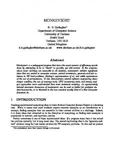
(a) Liquidation value is well predicted by traded prices.

(b) Previous liquidation values were less predictive.

Figure 1: Comparing two predictors of liquidation value. The dashed lines are the ideal y = x dependence; different symbols represent different markets. the previous trading period). Prizes were awarded twice: once after the second period of trading, and once after the fifth period of trading. Six prizes were raffled off each time, based on a trader’s rank and account value in each period. To illustrate, consider the 5th period prizes, which used trading performance in periods 3,4 and 5. The first prize, which was an iPod shuffle, was raffled off between 9 possible winners determined by the the top three accounts from each of the three prior periods. The probability that an account would win the prize was proportional to its account value. If the same account featured multiple times in the top-3, it had “multiple chances” to win the prize, thereby effectively increasing the probability of winning the prize. This was our mechanism to encourage participants to do well in every trading period. An alternative is to allow carry-over of previous account values. We opted for the reset mechanism because it allowed every account a chance in subsequent periods even if it did badly in prior periods. In the same way, the top 5, 10, and 20 accounts in each period were eligible for the 2nd, 3rd and 4th prizes respectively. Trading Periods 1-2 3-5

1st $69 $150

2nd $49 $100

Prizes 3rd 4th $40 $30 $60 $40

5th $20 $20

6th $20 $20

Table 1: The value of awarded prizes. Again, if an account featured in the top 3 accounts of a period, it was eligible for all the prizes; similarly, if an account featured in the top 5 (but not top 3), it was eligible for all prizes but the top prize, etc. The fifth prize was a participation prize awarded uniformly at random to one of the top 50% of traders in each period. The sixth prize was used to encourage participants to rate their professors and was drawn using probabilities proportional to the number of times a trader provided ratings. The prizes were awarded from 1st to 6th, with the restriction that once an account was awarded a prize, it became ineligible for any subsequent prize. The prize values are summarized in 4

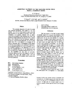
Table 1. From a theoretical standpoint, these incentives create complex utility functions. We could instead have awarded prizes with probability proportional to a trader’s total account value. However, making such a scheme sufficiently rewarding was not practical given reasonable constraints on the value of awarded prizes; rank order incentives such as those used in the IRM can be significantly more effective than proportional payments [17]. Simply paying participants based on their performance without vastly increasing the total amount awarded would likely have been demotivating [11]. While linear rewards for participation would seem to at least yield simple incentives, even this does not occur in practice, as other motivations are found to have a significant impact on experiment participants [16]. Anecdotally, students trading on the markets said they were far more willing to participate actively in pursuit of a high position on the leaderboard and a possible prize than they would have been with linear incentive schemes, either probabilistic or deterministic. Another point to note is that Luckner and Weinhardt [17] suggest that rank-order incentives were more effective than proportional payments in their experiments because reduced risk aversion among participants encouraged trading and made the markets more efficient. Similarly, a reduction in risk aversion may have played a part in encouraging extra trading on the IRMs, but this may also have increased noise trading, leading to greater volatility. Finally, we should note that rank-order incentives suggest different strategies for manipulation and collusion than proportional payments (see Section 4.1), but intrinsic motivation and ethics may play a bigger role than the precise monetary incentives. Ratings. Students taking one of the ten subject classes were given keys at the beginning of the semester which enabled them to rate their instructor at the end of each trading period. Each student who registered a key was sent a reminder email for each trading period. For the first period, rating was done through the same website as trading; for the remaining four periods, students could also rate directly from their reminder email. Initially, rating could be either thumbs-up (100%) or thumbs-down (0%), but a neutral option (50%) was added beginning with the third period. The initial limitation reflected the idea that only 0 and 100 were rational choices for traders seeking to maximize their wealth; we relaxed this limitation in response to feedback from students who did not want to rate their instructor either positive or negative. The liquidation value ∈ [0, 100] of a market was the average of all ratings cast for the associated trading period. The distribution of liquidation values is shown in Figure 2. Trading Interface and Microstructure. Traders interacted with the markets by placing market orders through the interface shown in Figure 3. Traders were presented with a full history of traded prices and liquidation values for each security, along with links to the associated course website. They were also shown the current (spot) price of the security, and could place a market buy or sell order for a desired quantity – they would then receive a price quote for their entire order, and were asked to confirm. For the first two periods, users started with 50000 units of virtual currency and 50 shares of each market. For the final three periods, users started with 100 shares of each class and the same amount of currency. Price quotes were generated using two different market making algorithms (only one algorithm was used for any given market during a particular trading period). We used an implementation of Hanson’s logarithmic market scoring rule (LMSR) [12] with a b parameter of 125 (restricting loss to 8664.34 in any given period)3 , and an implementation of the Bayesian Market Maker (BMM) 3 From a market making perspective, a real-valued dividend ∈ [0, 100] is equivalent to the more typical 0-1 dividend, modulo a constant factor; the extreme values of the dividend determine loss bounds where applicable on inventory-

5

Figure 3: Trading Interface

Figure 2: Distribution of instructor ratings

described by Brahma et al [4]. Both market makers are initialized at the beginning of a trading period so that the quoted price in each market is the same as the close of the previous trading period. Section 5 provides more details on the market making algorithms and compares their behaviors. Market Participation. Overall there were 226 registered users, with registration limited to current RPI students, faculty, and staff. Of these, 198 users made at least one trade during the experiment. Participation declined as the experiment progressed, with 117 active traders in the first period and only 33 in the fifth period. Rating was more steady, peaking at 93 raters during the second period, but never dropping below 70 raters during any period (see Appendix B). The backgrounds of participants were mixed: from undergraduates studying physics to faculty in computer science.

3

Information Content of Prices

Prediction markets attempt to aggregate information and to incentivize the dissemination of information that is otherwise difficult to obtain. The obvious question is whether traded prices in the IRM provide any new information about future instructor ratings. If traders simply provide a noisy realization of the previous rating (dividend), for example, then the prices themselves do not provide useful dynamic instructor feedback, other than, perhaps, getting students engaged enough to actually provide the ratings. Do the markets have predictive power?

3.1

Predictivity of prices

Figure 1(a) answers this question in the affirmative. In the figure is a scatter plot of the upcoming liquidation value versus the average traded price. Different markets are referenced with different symbols. Also shown is the ideal outcome (the line y = x). Modulo noise in the data, there is good agreement between the data and the ideal line. We use an average traded price because prices are noisy and averaging can provide a better proxy for the market value than the price of any single based market makers.

6

executed trade.4 Such smoothed prices were significantly more predictive than previous liquidation values, with a four-day average price yielding an R2 value of 0.58, while previous liquidations produced an R2 of 0.48. This finding is robust to different averaging windows for prices and different aggregates for previous liquidations; see Appendix C for details. We also note that there was a slight optimistic bias of approximately 5.0% in the 4-day average market price as a proxy for the future liquidation value; this was also true for the prior liquidation value, which had a bias of approximately 3.4%. Neither of these optimistic biases were statistically significant, but it does suggest that there was a systematic downward drift in ratings through the semester which was not captured by the prices (nor the prior liquidation value). To further validate that market prices are a better predictor of future liquidation values than prior prices, we ran a regression using both the previous liquidation value and the market price as independent variables in the following linear model: Liqs,ρ = β1 Liqs,ρ−1 + β2 Prices,ρ + α

(1)

where Liqs,ρ is the liquidation value of market s in period ρ, and Prices,ρ is the 4-day average market price before liquidation. The sample size for this regression is 40, since we have no previous liquidation value for securities in the first period. The significance of the previous liquidation value at the p = 0.05 level disappears when price is included in the linear model above, showing that previous liquidation value provides no additional information beyond price in this regression (see Appendix A for the regression results). Of course, traders may be (in fact, they almost certainly are) learning from previous liquidation values and incorporating that information into prices. This result is robust with respect to the choice of how price is smoothed. For Prices,ρ equal to the 4-day average price, we find that β2 is the only statistically significant coefficient (at p < 0.05). The results are qualitative unchanged when adding random effects controls for per-period and per-stock variations.5

3.2

Insider trading and the sources of information

Having shown that prices are predictive, we would like to know where the new information is coming from. While this is sometimes done by looking at the trade prices of different types of traders, that methodology is more appropriate for markets with limit orders. In a market-maker mediated market, it makes more sense to look at the directions of trades. Consider a single trade on the IRM: either this trade moves a price toward the corresponding instructor’s future rating, or away from it. By examining the set of all IRM trades in this manner, we can get an idea of the information revealed by groups of traders. We would expect that in-class traders, since they determine instructor ratings, would provide more information than out-of-class traders. Indeed, inclass traders traded toward the future liquidation 53.9% of the time (95% confidence interval 53.0% to 54.8%), while out-of-class traders traded toward the future liquidation only 52.5% of the time (95% confidence interval 52.3% to 52.8%). The difference is statistically significant (p = 0.015). This tells us that in-class traders brought more information to the IRM. However, we know that previous liquidations are a good predictor of future liquidations; how many of these trades are simply based on old information? 4

Collecting information from prices in this pilot deployment would have been difficult to do in real time because of volatility, especially when using LMSR as the market maker. One could combat this by increasing the loss tolerance of LMSR, effectively performing smoothing with the market maker itself. 5 We added αs and αρ as random effects, assumed to be normally distributed with mean zero, representing random per-stock and per-period variations respectively.

7

To determine which traders bring new information to the IRM, we can examine trades that occur at prices between the previous liquidation price and the future liquidation price. In such situations, if insiders are truly the sources of fresh information, we would expect them to trade more in the direction of the future liquidation, while others trade more in the direction of the last liquidation. Examining the data confirms this hypothesis. In situations where the execution price was in between the last liquidation value and the next liquidation value, in-class traders traded toward the future liquidation 53.5% of the time (95% confidence interval 51.7% to 55.2%, so also significantly more than 50% of the time). Out-of-class traders favored the previous liquidation, trading toward the future liquidation only 47.7% of the time (95% confidence interval 47.0% to 48.4%, so significantly less than 50% of the time). The difference is, of course, statistically significant (p = 7.1 × 10−7 ). This is compelling evidence that out-of-class traders were mostly trading on old information, and the markets serve to disseminate the inside information of in-class traders to the world, and provide feedback to instructors in doing so.

3.3

Qualitative features of prices

Figure 4 shows the traded prices and liquidation values for a selection of markets (traders saw this information in a similar format, although they were not aware of which market maker was used in which period). The figures highlight certain interesting qualitative features of the price processes. First is the effect of volatility, which may make the instantaneous price a less useful piece of information for the instructor at any point in time than a smoothed version of the price, as discussed earlier. An alternative would be to use a less volatile market making scheme (different parameters or a different algorithm). In fact, volatility does appear to be significantly less for markets using BMM (a relatively recent Bayesian Market Maker [4]), which we discuss later; this lower volatility does not come with any loss in predictive ability of the resulting prices. Second, prices often move towards the previous liquidation right after that value is revealed, without moving all the way there. We see this behavior clearly in Course 1, especially during periods four and five. Two of the IRM classes always liquidated at a value of 100, and in these classes the security prices slowly converged to 100; the slow rate of convergence is probably because the incentive to buy a security near 100 even given a sure liquidation at 100 is very small. Summarizing the evidence from this section: the markets are useful and predictive, providing information on future ratings that instructors will receive. We find strong evidence that most of the useful new information is added by in-class traders. Meanwhile it appears that out-of-class traders help in providing market stability by trading toward previous liquidation values, offsetting large noise trades.

4

Trading and Rating Behavior

One of the unique benefits of the IRM is that we have data on both the trading and rating behavior of the participants. This allows us to explore issues in market manipulation and trader behavior in ways that were previously not possible. For example, Section 3 presents evidence not only that the IRM succeeded in its primary goal of providing dynamic predictive information on how a professor is doing, but also that this information was mostly provided by students enrolled in the class. Here we look more deeply into the behavior of users.

4.1

Insiders, Manipulation, and Collusion

Traders who had rating credentials in a market (in-class traders, or insiders) could both trade in the market and affect the dividend through their rating. Therefore, not only did they have better 8

Figure 4: Price charts and liquidation values for selected markets, with line style indicating the market making algorithm. Each trade is plotted according to its transacted price with no smoothing. information on the professor being traded than other participants, but they had the opportunity to explicitly choose how to rate the professor based on their position in the stock. We define “manipulation” as situations in which students provide a rating they do not truly believe in order to maximize their profits from the IRM. There were plenty of opportunities for manipulation: several classes had only 3-5 raters, and information on how many ratings contributed to a particular liquidation value was made easily accessible on the trading interface (along with the prior liquidation values), allowing raters to estimate their impact on a market’s liquidation. Of course, knowing if manipulation actually occurred is difficult, but we provide several pieces of data that make the case that there was little manipulation. First, on a global scale, it is interesting to know whether the ratings students gave using the IRM interface (or direct email links) corresponded well with what they actually thought of the class. Since seven of the ten classes were in the Computer Science Department, we were able to

9

measure the correlation of IRM ratings with the official end-of-semester student evaluations.6 We averaged the ratings and prices of periods 3-5 in the IRMS. The coefficient of correlation of the IRM ratings to the official ratings for these 7 classes was 0.86, and the coefficient of correlation of the IRM prices averaged over these periods with the official ratings was 0.75. The strong correlation between IRM ratings and official ratings validates the usefulness of our markets in terms of a real benchmark that is “outside the system,” and also indicates that students were rating honestly in the IRMs, and that we do not need to worry about experiment-wide misbehavior. What about more limited manipulation? There has been both theoretical [14] and experimental [15] work on quantifying the potential effects of manipulators on prediction markets. Our experiment differs in that the objective of a potential manipulator is not known to traders. Consider a group of students in a given course who decide to manipulate a security to their advantage; either the group can decide to rate high and buy the security discreetly, or rate low and sell the security discreetly. In the first case traders make money directly from the artificially high liquidation value of the security, whereas the second case increases their wealth in comparison to other traders. Since several prizes were allotted based on relative account values, there were incentives for collusion of either form, but the behavior was not explicitly incentivized as in [15]. We considered any group of raters who both gave the same rating and made a significant amount of money (1000 virtual currency each) trading the associated security during a given period as candidates for having colluded. Many such potential collusions can be better explained as coincidence when examining the rating records of participants; raters who consistently gave the same rating were probably not being manipulative, as market prices would quickly adjust. This leaves a very short list of potentially collusive groups, described below. It is likely that some unsuccessful attempts at collusion went unobserved. We observed collusive behavior in course 3 during period 4. A group of 3 raters together made about 9000 in virtual currency by selling course 3’s security and rating the course low. Course 3 had 15 raters during this period, making it a surprising candidate for manipulation compared to the courses with 2 or 3 raters. However, these 3 students did control 20% of the liquidation value; since most liquidations were between 60 and 100 (see Figure 2), this was enough for the manipulators to reduce the security’s price significantly below the market’s expectation. This liquidation was Course 3’s lowest, although it is not apparent from the liquidations alone that manipulation was involved (see Figure 4). Pairs of raters made somewhat smaller amounts of virtual currency in several other markets, but it is not clear if intentional manipulation was involved. More surprising than the observed manipulation in the IRM was its relative scarcity. Most markets did not see any successful collusion based on the criteria that raters both made money and rated together during a given period. For markets with many raters, the incentives for manipulation may not have been high enough; capitalizing on noise traders takes much less effort than organizing a large collusion. For classes with very few raters, however, the incentives for manipulation by even a single rater acting alone were significant. Perhaps students did not understand the opportunities for manipulation, or perhaps giving accurate feedback was more important than winning prizes for some raters. We note that the potential for manipulation was not limited to groups or to simple rating manipulation. Examining the trading records of raters who made more than 1000 virtual currency trading in a given security during a given period, however, seems to indicate that such opportu6

In order to prevent loss of confidentiality for the instructors, we gave information on the IRM ratings and prices to the Department Head, who ran the correlations against end-of-semester student evaluations.

10

nities where not successfully exploited; we do not observe significant shifts in trading activity by these raters. Manipulation by non-raters seems significantly less likely given the relative lack of information and influence. On occasion, raters sold all their shares in a market, and still rated a professor as 100; this is surprising, because, given that they have no share holding, and that prizes are distributed according to relative account value, it is always in the best interest of such a profit seeking rater to rate the professor at 0, thereby reducing the value of all other traders. The fact that this did not happen suggests that there were perhaps not enough incentives for raters to behave in this way; or, perhaps raters felt a genuine obligation to give useful feedback to the professors. Somewhat more generally, Figure 5(a) shows the extent to which a user’s position in a security correlates with that user’s rating. For the most part, raters seem to “trade their beliefs”: users with a large holding in a market tended to rate the associated class highly, while users who sold all their starting shares of a security generally rated negatively. There is an anomaly around percentile 20, where we see unexpectedly high ratings. This anomaly represents traders who sold most of their shares, but nevertheless rated their instructor highly (perhaps the opposite of manipulation, as we define it above). These traders explicitly decreased their chances of winning prizes in this experiment by rating positively. Several prizes were raffled off based on relative account values, and no short selling was allowed; thus, raters who sold most of their shares had reason to believe that other traders would benefit disproportionately from a positive rating. We can conclude that either this group of traders were irrational, or they were motivated both by virtual currency and by giving their instructors feedback. Digging a little deeper, we find that these traders were actually among the more effective traders in terms of profits, perhaps exploiting a slight optimistic bias among the general trading population, but they simply decided not to use (or abuse) their rating privilege to their advantage.

4.2

Incentivizing Rating

Does trading regularly incentivize eligible students to rate? Figure 5(b) shows some evidence that answers this question affirmatively: more active traders were much more likely to rate. However, this alone does not support causality in either direction. While we cannot rule out the possibility, there is no a priori reason to believe that some underlying characteristic would increase propensity to both trade and rate; trading is a competitive activity, while rating is more social. Therefore, we hypothesize that this is an additional way in which the IRM adds value, since the ratings are useful feedback to the instructor independent of the information content in the prices. There is also a small group of users who did not trade, and yet did provide ratings – clearly these students were motivated by providing feedback rather than by using their rating to maximize expected prize winnings.

4.3

In Versus Out-of Class Biases

Many prediction market experiments report on the existence of interesting biases in the trading population. For example, Google’s corporate prediction market revealed a significant optimistic bias among new employees, diminishing as they became more experienced [7]. In our setting, a particularly interesting question is whether students who are enrolled in a class behave differently than others, in terms of their trading behavior. Our main finding is that traders who were in a class displayed a statistically significant optimistic bias about the value of the market for that class. However, the effect is entirely due to the first period of trading, and disappears thereafter, indicating that once students have data, they trade based more on that data than their perception 11

(a) Raters who gave a higher rating tended to have a larger number of shares in the market they were rating.

(b) Frequent traders are more likely to rate their professors.

Figure 5: Rater behavior, with about 87 raters per period. (Regression lines also shown.) of how much other students in their class like the instructor. We define trading bias for a user trading a particular market as the difference between the user’s valuation of the market and that market’s liquidation value. To estimate the user’s valuation, we use the midpoint of the user’s execution prices: the average of the user’s highest buy order and lowest sell order. Bias =

min(Sell) + max(Buy) − Liquidation 2

(in about 29% of cases, the trader’s highest buy price was higher than the lowest sell price; removing this data does not significantly affect our results). We wish to model this bias in terms of an overall bias across all users and an additional in-class bias among students taking a class corresponding to the market. Consider the following linear model: Biass,u = βInClasss,u + α

(2)

((s, u) index the market and user; we treat a different trading period as a different market); InClasss,u is an indicator variable which is 1 when user u is in the class associated with market s and 0 otherwise; α is the entire population bias, and β is the additional in-class trading bias. Across all periods (1899 samples from 101 raters), we see a small but statistically significant inclass optimistic bias (β > 0), but the entire population bias α is not statistically significant. Fitting separate models to each period (see Appendix A), we see a significant optimistic in-class trading bias during the first period, followed by no statistically significant in-class bias during subsequent periods. Additionally, we find that the above in-class trading bias is not explained by the rating records of biased traders. Consider a small modification of the above model: Biass,u = βRates,u + α 12

(3)

(a) Successful traders typically made many small trades.

(b) Approximately Cauchy wealth distribution. (Dashed line is a fitted Cauchy distribution.)

Figure 6: Trader wealth, with about 60 traders per period. Rates,u is the value of user u’s rating for the course represented by market s, with possible values 0, 50, and 100. Here we only considered traders who were in the course they traded. Fitting the model across all periods (120 samples), there is again a statistically significant in-class optimistic bias (now represented by α) with a p-value 0.012, but we cannot rule out the possibility that there is no rating effect β (p = 0.134). Additionally, β was not statistically significant when fitting the model to each period individually. The results of models (2) and (3) are robust to per-user and per-market random effects.

4.4

Trading Strategies and Profits

Traders varied wildly in their activity levels, strategies, and apparent rationality. While some amassed large quantities of virtual currency by frequently monitoring for mispriced securities, others seemed eager to cause as much havoc as possible while divesting themselves of their entire initial capital. Figure 6(a) shows the number of trades and the number of shares traded per user and per period, grouped by the user’s account value at the end of that period. We see that the defining feature of the most successful traders was activity; while they did trade more shares overall, they did so in almost twice as many transactions as the less successful traders. The worst traders also stood out, making a moderate number of massive trades. The most successful traders tended to trade in a large range, with low average buy and high average sell prices. We see that the most successful traders were those who executed the highest quantity of strategic trades; they capitalized on security values brought to illogical prices by noise traders. From an equity and efficiency perspective, this suggests that a market that also allows traders to place limit orders may offer some advantages in rewarding traders for bringing new information to the market, because such traders would not have to continuously poll the markets for erroneous prices. There was no significant difference between the wealth earned by traders in markets for classes in which they had rater credentials and those they did not. Successful traders who were in at least one IRM class, however, made most of their wealth in markets where they did not have rater

13

credentials; such markets were much more numerous. This may again indicate that searching for erroneous prices was more lucrative than trading mostly on specific information. Note that this does not imply that in-class traders did not add useful information to their class markets, just that they made more profit on other trades, in addition to the information they added to their classes. Figure 6(b) shows the distribution of profits among traders, calculated per (period, security) pair. The realized distribution is well fit by a Cauchy distribution. Interestingly, the shape parameter of the distribution (γ ≈ 525) is not significantly affected by the particular market maker used, although the market maker does affect the location parameter: with BMM (x0 ≈ −22) making more profit than LMSR (x0 ≈ 33). It is worth noting that LMSR still made money overall; the median trader made a small profit, but the mean trader profit was negative. In line with the discussion above, the majority of traders either made or lost a relatively small amount of money in a market during a given period. However, some traders took huge risks on a single market; many of these risks did not pay off.

5

Effects of Microstructure

The IRM is a powerful platform for testing the effects of different microstructures on price dynamics. We tested two different market-making algorithms. Brahma et al [4] develop a Bayesian Market Maker (BMM) (building on [8, 9, 10]), and compare with Hanson’s Logarithmic Scoring Rule (LMSR) market maker [12]. They find that BMM can offer comparatively higher price stability and smaller spreads than LMSR without suffering losses in expectation. On the flip side, LMSR comes with a strong loss bound, while BMM may occasionally take high losses. We provide additional evidence for these conclusions. The experiments in Brahma et al [4] were short 10-minute trading sessions based on an onscreen random walk; traders competed to quickly take advantage of new information. Long running markets like the IRM pose a different challenge for market making algorithms, because they are more prone to manipulation, especially by trading bots and collusive traders, who have more time to find and exploit holes in the market maker. In live testing, prior to deployment, we enhanced BMM in several ways (reported below) to prevent manipulation. We did not encounter any problems with manipulation, although several students spent a lot of effort attempting to hack the IRM in the first several weeks.7 Description of LMSR and BMM. LMSR is a purely inventory-based market maker. For a single security with payoff in [0, 1], the spot price at an inventory level qt is given by p(qt ) = eqt /b /(1 + eqt /b ), and the cost for a change Q in the inventory is  where b is a positive parameter,  C(Q; qt ) = b ln (1 + e(qt +Q)/b )/(1 + eqt /b ) . Thus, for a buy or sell order of size Q at an inventory level qt , the market maker quotes a volume weighted average price (VWAP) |C(Q; qt )/Q| where Q is positive for buys and negative for sells. The inventory is updated to (qt + Q) only if the trade is accepted, and the market maker waits for the next order. Note that, in our implementation, all these quantities are multiplied by 100 to keep the prices in the range [0, 100]. BMM, an information-based market maker, maintains a Gaussian belief distribution N (µt , σt2 ) for the value of the market; the spot price is equal to the mean belief µt . The underlying assumption is that trader valuations are normally distributed around the true value V . A fixed trade size parameter (α) determines quoted prices: every buy/sell order of size Q is imagined to be a sequence 7

There were several instances of users repeatedly querying the market maker with small trade sizes, high frequency buying, selling and canceling of orders, as well as fake large blog and wiki posts that brought the site to a crawl. The attempted trading manipulation had no effect, while the website issues were fixed as we discovered them.

14

Market maker LMSR BMM

#Periods 35 15

Avg. profit 1341.67 8273.13

Max loss -5298.58 -13763.40

Std. dev. of prices 8.6 3.0

Dev. from liq. 16.9 9.6

Table 2: Overview of statistics for LMSR and BMM of k = dQ/αe independent mini-orders of sizes {αi }ki=1 which are all α except possibly the last one. The market maker then quotes a VWAP and updates its state depending on the trader’s decision (acceptance/cancellation); the precise updates are non-trivial, but efficient (see [4] for details). Even though the Bayesian belief updates converge, BMM can adapt to market shocks, where the market’s value changes dramatically. To do so, BMM maintains a “consistency index” that quantifies how consistent the trades in a window of size W are with the current belief. When trades are inconsistent with the belief, the belief variance rapidly increases, allowing quick adaptation. LMSR is simple and loss bounded: the loss is at most b ln 2. Moreover, being inventory-based, it is difficult to manipulate; and, assuming rational traders who learn consistently from prices, an LMSR-mediated market converges to a rational expectations equilibrium. Though the loss is bounded, LMSR does typically run at non-zero loss. One drawback is that a single parameter b controls various aspects of the market such as the loss-bound, liquidity, and adaptivity; therefore, achieving a trade-off can be difficult. Moreover, Brahma et al find (and we confirm here) that if the beliefs of the trading population do not converge, prices can be very unstable. BMM, on the other hand, is not loss-bounded but makes much less loss in expectation while providing an equally liquid market. Moreover, in the absence of market shocks, BMM’s belief (and hence the spot price) converges owing to a monotonically decreasing variance, even if the traders maintain heterogeneous valuations. Exploiting BMM. The variance of BMM’s belief distribution determines its spread. A simple implementation can be manipulated by artificially tightening the spread, with a sequence of alternating small orders followed by a large order to exploit the low spread. To avoid this, we perform inference on BMM’s variance parameter only once for each trader unless an intervening trader also places an order. This idea can be easily extended to pairs of colluding traders, but could suffer from Sybil attacks. Such manipulation strategies are highly non-obvious, and, further, we limit traders to a single account by requiring an institute email address for authentication. Ultimately, exploitation of BMM did not become an issue. Comparison of Market Makers. We confirm the major findings of Brahma et al ’s previous comparison of BMM to LMSR. In essence, BMM offers more stable prices (see Figure 4 and Table 2), while making higher profits and maintaining lower spreads (see Table 2). We set LMSR’s b parameter to 125; by increasing b one can get lower spreads and more stability, but at the expense of other tradeoffs. For example, the b parameter of LMSR is an explicit market subsidy, increasing not only the loss bound but the expected loss of the market maker in reaching a given equilibrium price. Since LMSR actually made money on average, this could be an acceptable tradeoff. BMM already made more money on average in the IRM, however, and so comparing volatility is quite reasonable. It is interesting to note that the median trader made money when trading with LMSR, although the mean was below 0, whereas both the mean and median traders lost money with BMM. The volatility of prices and the deviation from the future liquidation value suggest that not only was the BMM price more stable than that of LMSR, it also provided a better estimate of the liquidation value. These results are robust and significant when regressing with per-security random effects

15

(see Appendix A).

6

Discussion

The Instructor Rating Markets are a proof of concept for the use of prediction markets in soliciting dynamic feedback. The IRM is a platform for studying the behavior of insiders and potentially manipulative participants in unprecedented depth. Despite using a simple market microstructure with only market orders, and running on a small scale, with only a few dozen active traders and 3-25 raters per class, market prices were predictive of instructor ratings. Further, instructor ratings received through the IRM system were very highly correlated with official institute end-of-semester evaluations. It is clear that students in a class were the ones injecting the most useful information into prices. At the same time, while raters had incentives to manipulate the dividend, individually or in collusion with others, surprisingly little of this type of behavior was observed. In fact, many raters acted contrary to their purely pecuniary interests in order to provide useful feedback to instructors via their ratings. Trading was also a motivating factor in the rating process, ensuring continued participation by raters. Our deployment also provides a platform for comparison of market microstructures, which we use to empirically validate a Bayesian Market Maker. Future deployments with limit orders and different parameter settings may lead to better outcomes with less smoothing of price necessary to provide useful dynamic feedback. Our results are in line with earlier work [17] which suggests that rank-order incentives limit risk aversion, potentially increasing market accuracy at the cost of increased volatility. The success of the IRM despite significant volatility from noise traders is a validation of the potential of prediction markets even in small settings with complex incentive structures. At the same time, a larger deployment across more classes and students may provide even more predictive power and more useful feedback to instructors. Acknowledgements. We are particularly grateful to Professors B. Cutler, K. Kar, H. Newberg, M. Goldberg, C. Varela & A. Wallace for their participation in the IRM experiment, and Prof. M. Hardwick for his support of the project and running correlations for us with official evaluations. We also thank all the traders who participated anonymously! This research is supported by an NSF CAREER award (IIS-0952918) to Sanmay Das. Malik Magdon-Ismail is partially supported by U.S. DHS through ONR grant N00014-07-1-0150 to Rutgers. The content of this paper does not necessarily reflect the position or policy of the U.S. Government, no official endorsement should be inferred or implied. The U.S. Government is authorized to reproduce and distribute reprints for Government purposes notwithstanding any copyright notation here on.

References [1] K.J. Arrow et al. Statement on prediction markets. AEI-Brookings Publication No. 07-11, 2007. [2] J. Berg and T. Rietz. Prediction markets as decision support systems. Inf. Sys. Front., 5(1): 79–93, 2003. [3] J. Berg, R. Forsythe, F. Nelson, and T. Rietz. Results from a dozen years of election futures markets research. Handbook of Exp. Econ. Results, 1:742–751, 2008. 16

[4] A. Brahma, S. Das, and M. Magdon-Ismail. Comparing prediction market structures, with an application to market making. Arxiv preprint arXiv:1009.1446, 2010. [5] Y. Chen and D. Pennock. A utility framework for bounded-loss market makers. In Proc. UAI, pages 49–56, 2007. [6] Y. Chen, S. Dimitrov, R. Sami, D.M. Reeves, D.M. Pennock, R.D. Hanson, L. Fortnow, and R. Gonen. Gaming prediction markets: Equilibrium strategies with a market maker. Algorithmica, pages 1–40, 2009. [7] B. Cowgill, J. Wolfers, and E. Zitzewitz. Using prediction markets to track information flows: Evidence from Google. Working paper, 2010. [8] S. Das. A learning market-maker in the Glosten-Milgrom model. Quant. Fin., 5(2):169–180, 2005. [9] S. Das. The effects of market-making on price dynamics. In Proc. AAMAS, May 2008. [10] S. Das and M. Magdon-Ismail. Adapting to a market shock: Optimal sequential marketmaking. In Proc. NIPS, pages 361–368, 2008. [11] Uri Gneezy and Aldo Rustichini. Pay enough or don’t pay at all. The Quarterly Journal of Economics, 115(3):791–810, 2000. [12] R. Hanson. Logarithmic market scoring rules for modular combinatorial information aggregation. J. Prediction Markets, 1(1):3–15, 2007. [13] R. Hanson. Insider trading and prediction markets. J. of Law, Economics, and Policy, 4: 449–463, 2008. [14] R. Hanson and R. Oprea. A manipulator can aid prediction market accuracy. Economica, 76 (302):304–314, 2009. [15] R. Hanson, Ryan Oprea, and David Porter. Information aggregation and manipulation in an experimental market. J. Econ. Beh. and Org., 60:449–459, 2006. [16] George Loewenstein. Experimental economics from the vantage-point of behavioural economics. The Economic Journal, 109(453):25–34, 1999. [17] Stefan Luckner and Christof Weinhardt. How to pay traders in information markets? results from a field experiment. Journal of Prediction Markets, 1(2):147–156, 2007. [18] A. Othman and T. Sandholm. Automated market-making in the large: the Gates-Hillman prediction market. In Proc. EC, pages 367–376, 2010. [19] A. Othman and T Sandholm. Decision rules and decision markets. In Proc. AAMAS, pages 625–632, 2010. [20] A. Othman, T. Sandholm, D. Pennock, and D. Reeves. A practical liquidity-sensitive automated market maker. In Proc. EC, pages 377–386, 2010.

17

[21] D. Pennock and R. Sami. Computational aspects of prediction markets. In N. Nisan, T. Roughgarden, E. Tardos, and V. V. Vazirani, editors, Algorithmic Game Theory. Cambridge University Press, 2007. [22] D.M. Pennock. A dynamic pari-mutuel market for hedging, wagering, and information aggregation. In Proc. EC, pages 170–179, 2004. [23] E. Servan-Schreiber, J. Wolfers, D.M. Pennock, and B. Galebach. Prediction markets: does money matter? Electronic Markets, 14(3):243–251, 2004. [24] J. Wolfers and E. Zitzewitz. Five open questions about prediction markets. Stanford GSB Wkg. Pap., 2004. [25] Justin Wolfers and Eric Zitzewitz. Prediction markets. J. Econ. Perspectives, 18(2):107–126, 2004.

A

Regression Tables

Price vs. Prior Liquidation. We fit the linear model in Eq. (1) using the IRM price and liquidation data. We show the results for two different smoothing windows for averaging the price (4 and 14 days). In Eq. (1) α is the prediction bias, and is never statistically significant; β1 represents the variations in liquidation attributable to the prior liquidation value; β2 represents variations in liquidation attributable to the average price. We observe that the significance of prior liquidation in the regression is negligible when smoothed price is also available as an independent variable. #Days 4 14

α est. 7.02 2.84

β1 est. 0.17 0.31

β2 est. 0.72 0.63

** *

Sample size 40 40

* p < 0.05; ** p < 0.01

Estimating in-class bias. We fit the linear model in Eq. (2) of Section 4, to estimate in-class biases. In Eq. (2), α is an overall bias; the additional in-class bias β is statistically significant in the first period, but not in subsequent periods. Period start date 09-15-2010 09-29-2010 10-13-2010 10-27-2010 11-10-2010

α estimate -11.26 2.34 4.48 6.09 -1.73

** * **

β estimate 2.43 0.97 1.14 1.65 -2.08

**

Sample size 625 499 345 219 211

* p < 0.05; ** p < 0.01

Comparing market makers. Let Stds,ρ be the standard deviation of the sequence of transaction prices for security s during period ρ. We also introduce a measure of accuracy for each market maker formalized as v u X 1 u LiqDevs,ρ = t (Liqs,ρ − t)2 ||Pricess,ρ || t∈Pricess,ρ

18

Where Pricess,ρ is the set of execution prices and Liqs,ρ is the liquidation value for security s during period ρ. LiqDevs,ρ measures the deviation of prices from the security’s liquidation value. Now, we can compare market makers using the following linear models: Stds,ρ = βIsBMMs,ρ + αs + α, LiqDevs,ρ = βIsBMMs,ρ + αs + α, where αs is a per-security random effect normally distributed with mean zero. IsBMMs,ρ is an indicator variable equal to 1 if BMM was the market maker for market s and 0 if LMSR was the market maker. Fitting the first model, we find that both α and β are statistically significant: α ∈ [6.7, 10.5] with 95% confidence (α ≈ 8.6), and β ∈ [−8.6, −2.8] with 95% confidence (β ≈ −5.6). We conclude that the prices in markets using BMM as market maker had a lower volatility. Fitting the second model to all of our price data, we find that α ∈ [13.5, 20.3] with 95% confidence (α ≈ 16.9) and β ∈ [−12.9, −1.8] with the same confidence (β ≈ −7.3). However, LiqDevs,ρ over an entire period is inflated for LMSR by its extra variance; while any given price from a BMM security was more likely to be close to that security’s liquidation value, BMM’s overall predictions were not necessarily more accurate than those from LMSR. Also of note is the fact that we did not tune the b parameter of LMSR which trades off maximum loss and volatility.

B

Activity Statistics Market 1 2 3 4 5 6 7 8 9 10

2010-09-29 2010-10-13 2010-10-27 Traders Raters Both Traders Raters Both Traders Raters Both 78 14 12 51 16 12 35 17 5 70 13 9 55 20 11 30 17 4 81 11 10 49 20 10 32 17 7 7 6 10 3 8 2 81 54 35 44 56 35 13 8 12 7 12 5 4 3 6 4 6 1 68 48 33 48 46 36 9 4 7 3 5 2 34 3 3 52 4 2 39 1 0 75 1 1 48 3 1 40 3 1 3 3 7 2 7 2 75 57 32 2010-11-10 2010-12-01 Market Traders Raters Both Traders Raters Both 1 22 12 3 19 13 4 2 22 15 3 20 14 4 3 27 15 7 23 17 5 7 0 6 1 4 20 18 5 27 11 4 22 11 3 6 22 3 0 27 4 1 7 22 5 1 16 4 1 8 20 2 0 25 2 0 19 3 0 23 1 1 9 7 3 7 1 10 18 19

There was a significant drop in trading activity over the length of the experiment, but rating activity was fairly steady. 19

C

Price Smoothing

Figure 7: Predictability of liquidation values using price history versus prior liquidation value across all 50 liquidations (10 securities in 5 periods). About 110 trades per day contribute to the smoothed prices. Figure 7 shows the R2 value from regressing the future liquidation value on the average traded price, for different averaging windows. As a baseline, we also report the R2 from regressing the future liquidation value on the most recent prior liquidation value 8 . Indeed, the prior liquidation value does give a good R2 , of about 0.48. However, the traded prices give an even better R2 , almost 0.58 when the averaging window is 4 days – the traded prices contain significant additional information regarding the upcoming dividend than does the prior dividend. Also, observe from Figure 7 that as we average over recent prices, the quality of the predictor improves; however, as the averaging window gets too large, the quality deteriorates, because stale information is now being incorporated. The quality of the price based predictor is, however, always at least as good as the prior liquidation value benchmark. Overall, there is clearly a trade-off between the noise when looking at a small number of trades and recency of information when looking at too large a number of trades.

8

Traders had all prior liquidation values available to them when making trades, but the most recent prior liquidation yields a higher R2 than several notions of historical average.

20