was the Benomad SdK 1.7 [1]. Fig. 10. The Real time acquisition system in STRADA. The GPS has been tuned in a 3-D only-mode to deliver reliable positions, ...
Integrated Navigation using GIS-based Information Philippe Bonnifait, Maged Jabbour and Véronique Cherfaoui Heudiasyc UMR CNRS 6599, Université de Technologie de Compiègne BP 20529 - 60205 COMPIEGNE cedex FRANCE Tel. +33 (0)3 44 23 44 23 - Fax +33 (0)3 44 23 44 77 {firstname.name}@hds.utc.fr Abstract This paper describes the usefulness of a GIS for integrated navigation of intelligent vehicles. In many applications, the use of GPS alone is not sufficient and needs the help of dead-reckoned sensors, map data and additional sensors like cameras or ladars (laser scanners). Geographical information can be used in two different ways. First, pre-existing features of the environment like roads can be used as constraints of localisation space. Second, the geographical information can include the landmark locations. The GIS can be used to manage this information. These two characteristics are described through the case study of a localisation system for urban areas.
1 INTRODUCTION Precise dynamic localisation with respect to a digital map is an essential task for Advanced Driver Assistance Systems (ADAS) and for intelligent vehicles. As a matter of fact, Geographical Information Systems (GIS) can contribute to the characterisation of driving conditions by providing important data like signposts, speed limits, or hazardous zones like schools, pedestrian crossings, etc. It is well known that GPS suffers from satellite outages and multi-tracks which can decrease significantly the availability and the precision of the delivered positions. This is particularly crucial in urban canyons for instance. To deal with such problems, positioning systems often rely on the integration of GPS and dead-reckoned or inertial sensors (odometers, MEMS - Micro-Electro-Mechanical Systems, gyrometers, etc.). Nevertheless, if a GPS outage lasts too long, the drift of the estimated pose (position and attitude) can become too large and unsuited for some applications, particularly in robotics where localisation is essential to carry out the task. On the other hand, the maps used in a GIS include information which can contribute to the localisation process itself. For instance, the description of the road-network can be used to localise a vehicle, even when the GPS signals are blocked. Another example is a cadastral map that can include the description of the roads and of the buildings. Such maps can be very detailed and their precision can be better than one meter. Finally, there are many localisation systems that rely on the use of extra exteroceptive sensors such as cameras, ladars (laser range scanners) or telecommunication-based systems (UMTS, wifi, etc.). A key common point of these systems is to use beacons, landmarks or features the location of which needs to be known. If these beacons have been localised or if they have been detected by aboard sensors, their coordinates can be managed in the GIS database. This landmark geographical information allows correcting the estimate of the pose during navigation. For instance, the curbs of the road can have been charted in a GIS map and sensed by a
camera or a ladar. The GIS can also be used as a tool to update existing landmark information. The aim of this paper is to illustrate the use a GIS for integrated navigation in the area of Intelligent Vehicles (ADAS or autonomous vehicles). We will describe a positioning method that relies on the use of differential GPS, odometry aided by a gyrometer and a road-map. In order to increase the precision and to correct the drift of dead-reckoning localisation, we will study the use of visual urban landmarks. We will illustrate the usefulness of a GIS to manage the different characteristics of geographical information in different layers. The paper is organised as follows. Section 2 concerns the use of pre-existing geographical information which acts as a constraint of localisation space. The case of charted roads is considered. The fusion of GPS, map information and odometry is done by an Extended Kalman Filter (EKF). Section 3 deals with the management of natural landmarks in a GIS layer for a precise localisation especially in urban environments. The management of key images information is described and analysed through experiments carried out with our experimental car.
2 USING CHARTED ROADS IN THE LOCALISATION PROCESS 2.1 Introduction Usually for automotive applications, a GIS database is a set of cartographic information provided by a cartographer like NavTeQ or TeleAtlas. This a priori known information is very useful for the navigation tasks like route guidance. Indeed, for this purpose, a scanty representation of the road network is sufficient: roads are described by linear lines which correspond to the central axis of the road. The localisation is forced by the lines: the position is obtained by a projection onto the lines. This is the mapmatching process.
central axis
Nodes
b Shape points
S
Fig. 1. Description of the roads in a usual map by nodes and shape points
In a different approach, the geographical representation of the road network can be used as positioning information with its own uncertainties. In such a context, the localisation problem can be considered as a Data Fusion problem in which several different information sources need to be combined in order to provide a more precise and reliable positioning system that is able to eliminate aberrant data for integrity purposes.
2
2.2 Fusion of GPS and dead-reckoning sensors Let consider the multi-sensor fusion of a GPS receiver, an odometer and a gyro with a road-map. If the GPS satellites signal is blocked by buildings, for example, the evolution model provides a dead-reckoned (DR) estimate, the drift of which can be corrected using the map information. The mobile frame is chosen with its origin attached to the centre of the rear axle. The x-axis is aligned with the longitudinal axle of the vehicle. The vehicle position is represented by (xk,yk), the Cartesian coordinates of M in a global frame (a projection of geographic data). The bearing angle is denoted θk. The evolution model of the vehicle is non-linear: Xv,k+1 = f (Xv,k ,Uv,k , γk) + αv,k (1) Where Xv,k is the vehicle state vector at the instant k, composed of (xk, yk, θk), Uv,k the vector of the measured inputs consisting of (∆k, wk), ∆k and wk being respectively the elementary distance covered by the rear wheels and the elementary rotation of the mobile frame. αv,k is the process noise and γk represents the measurement error of the inputs. αv,k and γk are assumed to be uncorrelated and zero mean noise. If the road is perfectly planar and horizontal and if the motion is locally circular, the evolution model can be expressed by: ⎧ wk ⎞ ⎛ ⎟ ⎪ xv, k +1 = xv , k + ∆ k . cos⎜θ v , k + 2 ⎠ ⎝ ⎪ wk ⎞ ⎛ ⎪ ⎟ ⎨ yv , k +1 = yv, k + ∆ k . sin ⎜θ v , k + 2 ⎠ ⎝ ⎪ ⎪θ v, k +1 = θ v, k + wk ⎪ ⎩
(2)
The values of ∆k and wk are computed using the odometer measurements of the rear wheels and a fibre optic gyrometer. The fusion of GPS and odometry is done by Kalman Filtering (Extended KF here but it could be Uncented KF [6]) which uses the prediction/update mechanism. In the prediction step, the car evolves using (2) and the covariance of the error is estimated. When a GPS position is available, a correction of the predicted pose is performed. In urban areas, GPS suffers from multi-tracks and bad satellite constellation (urban canyoning) that degrade the position that it delivers. So, when a GPS position is available, it is necessary to verify its coherence. For that, the Normalized Innovation Squared (NIS) with a chi-square distribution is used: a distance dm is computed between the GPS observation and the state vector. Let Yv be the observation vector, µv the innovation vector.
⎡1 0 0⎤ ⎡ xGPS ⎤ Yv = ⎢ = ⎢ ⎥ ⎥ . Xv + βGPS = Cv . Xv + βGPS ⎣0 1 0⎦ ⎣ y GPS ⎦
(3)
⎡x − x⎤ µv = ⎢ GPS ⎥ ⎣ y GPS − y ⎦
(4)
dm = µv . (Pµ)-1. µvT
(5)
Where (x, y) is the predicted position and Pµ is the covariance of the innovation.
3
If the computed distance dm is smaller than a threshold, for instance χ2(0.05,3), then the GPS measurement is assumed to be correct and a correction of the predicted pose is performed. Otherwise, the dead-reckoned pose provided by the evolution model is kept. Please, note that the GPS noise is not stationary. The GPS measurement error can be estimated in real time by using the NMEA sentence GST. This information is provided by the TRIMBLE AgGPS132 GPS receiver that has been used in the experiments.
2.3 Road selection In order to fuse Map information, we need to consider the road selection problem which consists in extracting from the GIS map the most likelihood segment using the estimated state vector. On Figure 2, the estimated pose is denoted by an arrow (representing the estimate of the heading) and a 95% ellipse under Gaussian hypothesis. The segments that are plotted have been extracted from the GIS road-map layer. There are different approaches to solve the road selection problem. Usually, the distances between the estimate and the nearest segments are computed. The segment that has the smallest distance and whose driving direction corresponds to the heading of the vehicle can be considered as the good one. 3100 3150 3200 3250 Y 3300 3350 3400 3450
2250 2200 2150 2100 2050 2000 1950 1900 1850 1800 X
Fig. 2. Illustration of the roads selection problem
A more reliable method can be obtained by fusing selection criteria as presented in [4].
2.4 Fusing the map information In order to fuse the map information, a matched point is built by projecting the estimated position onto the selected segment. The matched point can be used as a map observation (denoted Yvm) in order to correct the drift the DR estimate if the GPS is unavailable:
⎡1 0 0⎤ ⎡x ⎤ Yvm = ⎢ MAP ⎥ = ⎢ ⎥ . Xv + βMAP = Cv . Xv + βMAP 0 1 0 y ⎣ ⎦ ⎣ MAP ⎦
4
(6)
Another NIS coherence test is used to verify the map observation coherence before fusing it thanks to a Kalman filter correction stage. A key point relies on the quantification of the covariance of the map βMAP. An efficient way is to model the imprecision by a ellipse whose principal axle is collinear to the segment. The width of the ellipse is taken proportional to the width of the road (see Fig. 3)
Confidence Zone around the segment Step 2
Fusion (GPS, Odo) Step 1
Result of the fusion Step 3
Fig. 3. Illustration of the fusion of segment with the previous estimated position
2.5 Results Figure 4 presents a top view of a 4-km long experimental test performed in Compiègne. The map was an IGN Géoroute V2 data-base managed by the GIS software "Geoconcept". The DGPS receiver used was a Trimble AgGPS132 with an Omnistar differential correction.
End
Start
Fig. 4. View of the used IGN Géoroute V2 map. The trajectory of the vehicle is in bold
5
On Figure 5, the usefulness of the map information is illustrated. The path plotted with ‘o’ corresponds to the rough absolute positions provided by the DGPS transformed in the French Lambert coordinates system of the map. The ‘+’ path is the result of the fusion of the sensors with the road-map. On can notice that, as mentioned before, the result of the fusion does not match exactly with the roads (this can be easily seen in the roundabouts). -100 y (m)
DGPS Position -150
Corrected Position
-200 -250 -300 -350 -400
Right road
-450 -500 -550 -600 -550
-500
-450
-400
-350
-300
-250
-200
x (m)
-150
Fig. 5. DGPS positions, {DR, DGPS, map} fused positions 500
y (m)
DGPS Positions Corrected Positions DR only estimates
0
-500
DR estimated positions
x (m)
-1000
-1500 -1200
-1000
-800
-600
-400
-200
0
Fig. 6. Illustration of the drift of the DR estimates
6
200
x (m) 400
In the experience of Figure 6, a GPS outage has been introduced at the exit of the first roundabout (in the bottom). One can remark that in spite of the long DGPS mask (about two kilometers), the vehicle is correctly located. As a matter of fact, the final estimated positions stay close to the GPS points. One can see that the map observation corrects efficiently the drift of the DR localisation.
3 PRECISE LOCALISATION USING LANDMARKS MANAGED IN A GIS LAYER 3.1 Introduction For intelligent vehicles, there are many outdoor navigation applications which need a high precision localisation (ie around 10/20 cm). Real Time Kinematic (RTK) GPS is a very interesting candidate for this localisation purposes since it can reach few centimetres accuracy in real-time by using phase corrections broadcasted by base stations. Nevertheless, this technology is not adapted to vehicles that evolve in urban areas since the receiver needs to see at least 5 satellites with a good configuration (small DOP). Moreover, after the loss of the fixed mode, the system needs to solve the phase ambiguities problem which requires typically 30 seconds processing. A solution relies on the use of additional sensors installed aboard the vehicle like video cameras and ladars (laser range scanners). Indeed, they are well adapted to the sensing of natural landmarks, especially those of urban areas since they are very stable like, for instance, the buildings or the road features. The landmarks are characterized and localised in a learning stage during which the vehicle is driven manually. Afterwards, the vehicle is able to locate itself and control its movement near to the learned trajectory. Recent works (like the experiments performed by Royer et al. [7] using computer vision for instance) have proved the validity of such a concept.
3.2 Landmarks and enhanced geometry There are different kinds of landmarks that depend on the sensors used. They can be classified in the following categories: Active landmarks. Actives landmarks are beacons that include active components in order to transmit a signal. They mainly rely on the use of radio-frequency signals (GPS pseudolites, transponders stored in the pavement, Wifi antennas, etc.). Such landmarks are usually distinguishable from each other. In this case, sensors are receivers equipped with an antenna. Passive landmarks. They are artificial landmarks pertinently located in the environment for localisation purposes like magnets in the pavement or reflectors installed on post in curves, for instance. Natural landmarks. Natural landmarks are features of the environment detected by aboard sensors like video cameras or ladars [8]. They can correspond to characteristic points (edge of windows for example), road markings, roof of buildings, posts, curbs, sidewalks, etc. In cadastral maps, natural landmarks like road markings or curbs of the roads are sometimes charted by the cartographers. This enhanced geometry can be used for the localisation process.
7
3.3 Usefulness of a GIS As GIS is a set of tools and methods that manage and handle vectorized or raster geographical information, it is very useful to manage any kind of landmark. It is first useful to store the landmark information in dedicated geographical information layers added to the road-map (see Fig. 7). This information can be - enhanced geometry like cadastral information, - landmarks o actives or passive landmarks provided by a third entity, o natural landmarks sensed and characterized by the embedded localisation system. In order to build a precise GIS layer including natural landmarks, a learning stage is necessary. This can be done in a first passage.
Fig. 7. Geographical Information layers: road-map layer, enhanced geometry layer, landmark layer
A GIS is also interesting to retrieve the landmark information for the localisation each time the vehicle navigates in a known area. A difficulty of using local landmarks is the management and the structuring of a large amount of data for on-line navigation. Indeed, how to organize the landmark information for a vehicle that evolves in a large area including many roads? The usual answer to this question is to regroup landmarks in local maps, a local map being a set of landmarks put together because of i) memory constraints arising from the use of embedded systems, ii) the need to download or update a limited amount of data from a distant server and iii) the connections that exist between the landmarks, essential to compute a location. The GIS is very useful for the management of landmarks in local maps by benefiting from the roads description stored in the road-map database. Indeed, the management of landmarks for an intelligent vehicle can be performed with respect to the roads. In such a case, the absolute accuracy of a GNSS-based positioning is not crucial since the roadmap as a meter-level precision. Therefore, a single frequency GPS receiver fused with
8
dead-reckoned sensors and a map in order to handle satellites outages is sufficient, as indicated by the results of section 2.5.
3.4 Case study: management of visual landmarks In order to illustrate the concept of natural landmark, let consider visual landmarks with characteristic points 3D as used by Royer et al. [7] for the navigation of a Cycab using a mono-camera at video rate. These landmarks are characteristic points in images called Harris points [2] (cf Fig. 8). Thanks to these points, one can rebuild the 3D pose of the vehicle using a sequence of images (called key images) in which each landmark has been detected at least in two images. Please see [7] for more details.
Fig. 8. Example of detected visual features: Harris points
During a learning stage, the visual features are detected and stored in the corresponding additional layer of the GIS. Then, these features are extracted each time the vehicle navigates in the same area.
3.5 Map-Matching the key Images In the learning stage, dated images are acquired by cameras connected to an acquisition system, along with other sensors. This includes dead-reckoning sensors (odometers attached on the rear wheel and a KVH fiber optic gyrometer) and GPS data. In this stage, map-matched coordinates of the fused poses of the localisation algorithm shown previously are associated with the acquired images using timestamps in the same reference time coordinates. The map-matched point is the point called map observation in section 2.4. When this point is obtained, the ID (unique reference stamp in the database) of the road is retrieved. While the timestamp of the image to match falls between the timestamps of two positions belonging to the same road (they have the same ID), the geo-referencing of the image is done by a linear interpolation. If the two map-matched positions used to the geo-referencing have different ID, the nearest is kept and the image position is projected onto its segment. This simple strategy is well adapted in practice since the sampling rate of the matched position is significantly high (100 Hz used in the experiments).
9
3.6 Regrouping the images in local maps We proposed to regroup the images in local maps to facilitate their management. For this purpose, the use of road IDs is well adapted. Indeed, a road is a set of same ID segments with eventually a junction at its beginning or/and at its end. For the management of a GIS database, two different roads have necessarily different IDs. Moreover, each road can be one-way or double direction (this information is included in the road attributes). For one-way roads, a unique local map is built. It includes all the images matched to it. For double direction roads, two maps are built, one for each direction: E2W (East To West) or W2E (West To East). Figure 9 shows double direction roads with images associated to each direction.
Fig. 9. Associating images to road segments
3.7 Landmarks Extraction We consider now that the vehicle navigates in the environment learned in a previous stage. In the navigation phase, the system needs high precision for localisation. A centimetre-level precision is obtained when the vehicle can use the pertinent learned landmarks regarding the observed landmarks during navigation. The topic of this paragraph concerns extraction and selection in the additional GIS layer of pertinent landmarks at each time t of the navigation stage. The landmarks management for navigation consists in two parallel tasks: Local map extraction Visual landmarks selection The goal of the local map extraction is to obtain a vehicle pose with a precision in the order of one meter and then to find the appropriate local landmarks map stored in the GIS built landmark layer. The localisation algorithm is the same one used in the learning stage: it fuses GPS, road-map information with dead reckoning sensors. A first pose is computed and a map-matching is done using the fused pose. Then the road ID is retrieved. The road ID and the driving direction permit to select the adequate local map. If the selected local map is not the current local map, the visual landmarks are then loaded in the dynamic system memory. This supervisory task is repeated during the navigation process. It guaranties the transitions between two local maps. The local map extraction provides a local map mapj composed by a set of georeferenced visual landmarks as previously described. To obtain a precise localisation, the navigation process needs to use the landmark I having the nearest matched position 10
Xmapj,I. This is the landmark selection. In the experiments, the landmark which is selected is the one which is the nearest and downstream.
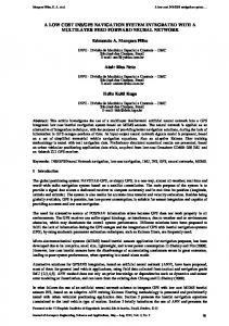
3.8 Experimental Results Real experiments have been carried out with our experimental car (see Fig. 10) in the downtown area of Compiègne (Fig. 11) using a KVH fibre optic gyro, an odometer input and a Trimble AgGPS 132 running with a geostationary differential correction (Omnistar). To test different technologies of cameras and various configurations, four cameras were connected to the acquisition system. Timestamped images were logged at the rate of 15 images per second. The used cameras were a fisheye one, a CMOS stereo pair (AVT Marlin F-131) and a Sony Firewire (DFW-VL500). The GIS software used was the Benomad SdK 1.7 [1].
Fig. 10. The Real time acquisition system in STRADA.
The GPS has been tuned in a 3-D only-mode to deliver reliable positions, by setting the DOP threshold to a low value, and the SNR threshold to a high value. Such tuning induces a reliable but intermittent positioning in urban areas.
Fig. 11. Overview of the NavTeQ road-map around the experimental field, with the itinerary plotted in red.
11
Figure 12 shows the vehicle localisation result (in bold) on the map (thin plot) in the urban environment. This localisation results had been used to map-match the acquired key images. The zoomed view shows key-images positions associated to road segments. 300
250
-50 -55
200 -60 -65
150 -70 -75
100
-80
50
-85 -344
-342
-340
-338
-336
-334
-332
-330
-328
-326
0
-50
-100 -350
-300
-250
-200
-150
-100
-50
0
50
Fig. 12. Map Matched results of the learning stage
Two weeks later, we carried out navigation experiences. Figure 13 shows in bold the localisation result and in thin red the segments where visual local maps has been previously acquired. To illustrate the visual landmark management, we extracted at each sample (in fact at each new image) the best key image for localisation as described before. 300 250
Unlearned road
200 150 100 50 0 -50 -100 -350
-300
-250
-200
-150
-100
-50
0
50
Fig. 13. Map-matched vehicle position for the key image retrieval needs
A graphical interface allows monitoring the localisation during the navigation process. The interface displays the map and adds two positions icons: the current matched position of vehicle is drawn with an arrow and the key image selected by the algorithm is represented by a squared point. Two additional windows display the current image and the selected key-image. At each position, the interface refreshes the current position, the current image and the key-image, if it changes. Figure 14 shows this interface.
12
Key-image
current image
Fig. 14. Real time graphical interface
The time stamped data was saved in order to analyze the results in post-processing and to verify that the extracted landmarks were the good ones. The route was 1.8 km long (travel time 6 mn). At each key image selection, the overlapping between key image and current image has been verified (except on the unlearned road where the system was able to detect that there was no key image). We consider that the selection is correct if the overlapping covers the half area of the images. The results give 98% overlapping when local map is available. The main errors come from the vehicle rotations at crossing road.
4 CONCLUSION For a precise and reliable localisation, the use of an integrated navigation system is a key issue. For intelligent vehicles, the localisation system can take profit of GPS data, proprioceptive sensors and GIS data. The a priori known GIS information can be made of networked roads or enhanced geometry maps. A data fusion method to localise the vehicle by using a road-map has been presented. It is important to notice that before using a GPS fix, its coherence is checked. This allows rejecting aberrant data arising from multi-tracks for instance. The robustness of the localisation is also improved by selecting the likeliest segment of the road-map. A map observation is then built to correct the errors. The resulting estimated position is not projected onto the likeliest road of the map, but closed to it. The GIS can also be used to manage enhanced geometrical information and landmarks. We studied the management of visual landmarks in a dedicated layer of the GIS data. They are regrouped in local maps attached to the roads. During the navigation 13
stage, these maps are retrieved and loaded in the memory of the localisation system and can be assimilated to a cache memory. These two applications illustrate the usefulness of a GIS for integrated navigation. The main drawback of existing GIS relies on their poor real-time capabilities. The Software Development Kit Benomad is well adapted for such an application since the Scalable Vector Format used is very efficient. ACKNOWLEDGEMENT
This research has been carried out in the framework of the project MobiVip supported by the French research program on transportation (PREDIT 3) from Dec. 2003 to Dec. 2006.
5 REFERENCES [1] http://www.benomad.com/ [2] Ch. Harris and M. Stephens, “A Combined Corner and Edge Detector” Proceedings of The Fourth Alvey Vision Conference, , pp 147-151. Manchester, UK. 1988 [3] M. Jabbour, V. Cherfaoui, Ph. Bonnifait, “Management of Landmarks in a GIS for an Enhanced Localisation in Urban Areas”, IEEE Intelligent Vehicle Symposium 2006, Tokyo, Japan, June 13-15, 2006 [4] El Badaoui El Najjar M., Bonnifait P. “A Road-Matching Method for Precise Vehicle Localization using Kalman Filtering and Belief Theory.” Journal of Autonomous Robots, Volume 19, Issue 2, September 2005, Pages 173-191. Kluwer Academic Publishers. [5] M. E. El Najjar and Ph. Bonnifait. “Intelligent Vehicle Absolute Localisation using GIS Information”. 16th IFAC World Congress, Prague, Czech Republic, from July 4 to July 8, 2005. [6] S. J. Julier and J. K. Uhlmann. “A New Extension of the Kalman Filter to Nonlinear Systems”. In / Proc. of AeroSense: The 11th Int. Symp. on Aerospace/Defence Sensing, Simulation and Controls./, 1997. [7] E. Royer, J. Bom, M. Dhome, B. Thuillot, M. Lhuillier, F. Marmoiton, “Outdoor autonomous navigation using monocular vision”. IEEE/RSJ International Conference on Intelligent Robots and Systems, pages 3395-3400, Edmonton, Canada, Aug. 2005. [8] Th. Weiss, N. Kaempchen and K. Dietmayer, “Precise Ego-Localization in Urban Areas using Laser scanner and High Accuracy Feature Maps”, IEEE Intelligent Vehicle Symposium, Las Vegas, USA, June 6-8, 2005. [9] W. S. Wijesoma, K. R. S. Kodagoda, and A. Balasuriya, "Road-Boundary Detection and Tracking Using Ladar Sensing", IEEE Trans. on Robotics and Automation, VOL. 20, NO. 3, pp.456-464 June 2004.
14