Integrating SLAM and Object Detection for Service Robot Tasks Patric Jensfelt, Staffan Ekvall, Danica Kragic, Daniel Aarno Computational Vision and Active Perception Laboratory Centre for Autonomous Systems Royal Institute of Technology, Stockholm, Sweden patric, ekvall, danik @nada.kth.se,
[email protected]
Abstract— A mobile robot system operating in a domestic environment has to integrate components from a number of key research areas such as recognition, visual tracking, visual servoing, object grasping, robot localization, etc. There also has to be an underlying methodology to facilitate the integration. We have previously showed that through sequencing of basic skills, provided by the above mentioned competencies, the system has the ability to carry out flexible grasping for fetch and carry tasks in realistic environments. Through careful fusion of reactive and deliberative control and use of multiple sensory modalities a flexible system is achieved. However, our previous work has mostly concentrated on pick-and-place tasks leaving limited place for generalization. Currently, we are interested in more complex tasks such as collaborating and helping humans in their everyday tasks, opening doors and cupboards, building maps of the environment including objects that are automatically recognized by the system. In this paper, we will show some of the current results regarding the above. Most systems for simultaneous localization and mapping (SLAM) build maps that are only used for localizing the robot. Such maps are typically based on grids or different types of features such as point and lines. Here we augment the process with an object recognition system that detects objects in the environment and puts them in the map generated by the SLAM system. The metric map is also split into topological entities corresponding to rooms. In this way the user can command the robot to retrieve a certain object from a certain room.
I. I NTRODUCTION During the past few years, the potential of service robotics has been well established. The importance of robotic appliances is significant both in terms of economical and sociological perspective regarding the use of robotics in domestic and office environments, as well as help to elderly and disabled. However, there are still no fully operational systems that can operate robustly and long-term in everyday environments. The current trend in development of service robots is reductionistic in the sense that the overall problem is commonly divided into manageable sub-problems. In relation, the overall problem remains largely unsolved: How does one integrate these methods into systems that can operate reliably in everyday settings. Since an autonomous robot scenario is considered, it is very difficult to model all possible objects that the robot is supposed to manipulate. In addition, the object recognition method used
has to be robust to outliers and changes commonly occurring in such a dynamic environment. Object recognition is one of the major research topics in the field of computer vision. In robotics, there is often a need for a system that can locate certain objects in the environment - the capability which we denote as ’object detection’. In terms of object recognition, the appearance based representations are commonly used, [1]–[3]. However, the appearance based methods suffer from various problems. For example, a representation based on the color of an object is sensitive to varying lighting conditions, while a representation based on the shape of an object is sensitive to occlusion. In this paper, we present an approach based on Receptive Field Cooccurrence Histograms, that robustly copes with both of the mentioned problems. In most of the recognition methods reported in the literature, a large number of training images are needed to recognize objects viewed from arbitrary angles. The training is often performed off-line and, for some algorithms, it can be very time consuming. For robotic applications, it is important that new objects can be learned easily. i.e. putting a new object in the database and retraining should be fast and computationally cheap. In this paper, we present a new method for object detection. The method is especially suitable for detecting objects in natural scenes, as it is able to cope with problems such as complex background, varying illumination and object occlusion. The proposed method uses the receptive field representation where each pixel in the image is represented by a combination of its color and response to different filters. Thus, the cooccurrence of certain filter responses within a specific radius in the image serves as information basis for building the representation of the object. The specific goal in for the object detection is an online learning scheme that is effective after just one training example but still has the ability to improve its performance with more time and new examples. We describe the details behind the algorithm and demonstrate its strength with an extensive experimental evaluation. Here, we use the object detection to augment our map with information about the location of objects. This is very useful in a service robot type application where many tasks will be of fetch-and-carry type. We can see several scenarios here. While the robot is building
the map it will add information to the map about the location of objects. Later the robot will be able to assist the user when he/she wants to know where a certain object X is. As object detection might be time consuming another scenario is that the robot builds a map of the environment first so that it can perform basic tasks and then when it has nothing to do it goes around the environment and looks for objects. The same skill can also be used when the user instructs the robot to go to a certain area to get object X. If the robot has seen the object there before it has a good initial guess of where to look for it, otherwise it has to search for it and can update its representation. By augmenting the map with the location of objects we also foresee that we will be able to achieve place recognition. This will provide valuable information to the localization system that will greatly reduce the problem of symmetries when using a 2D map. Further, along the way by building up statistics about what type of objects typical can be found in, for example, a kitchen the robot might not only be able to recognize a certain kitchen but also potentially generalize to recognize a room it has never seen before as probably being a kitchen. This paper is organized as follows: in Section II, our map building system is summarized. In Section III we describe the object recognition algorithm based on Receptive Field Cooccurrence Histogram. Its use for object detection is explained in Section VI-A. The detection algorithm is then evaluated in Section VI where we also show how we can augment our SLAM map with the location of objects. Finally, Section VII concludes this paper.
lamps. The M-Space representation allows the horizontal line features to be partially initialized with only its direction as soon as it is observed even though a full initialization has to wait until there is enough motion to allow for a triangulation. Figure 2 shows a closeup of a small part of a map from a different viewing angle where the different types of features are easier to make out.
II. S IMULTANEOUS L OCALIZATION AND M APPING One key competence for a fully autonomous mobile robot system is the ability to build a map of the environment from sensor data. It is well known that localization and map building has to be performed at the same time, which has given this subfield its name, simultaneous localization and mapping or SLAM. Many of todays algorithms for SLAM have their roots in the seminal work by Smith et al. [4] in which the stochastic mapping framework was presented. With laser scanners such as the ones from SICK, indoor SLAM in moderately large environments is not a big problem today. In some of our previous work we have focused on the issue of the underlying representation of features used for SLAM [5]. The so called M-Space representation is similar to the SP-model [6]. The M-Space representation is not limited to EKF-based methods. In [7] it is used together with graphical SLAM. In [5] we demonstrated how maps can be built using data from a camera, a laser scanner or combinations thereof. Figure 1 shows an example of a map where both laser and vision features are used. Line features are extracted from the laser data. These can be seen as the dark lines in the outskirts of the rooms. The camera is mounted vertically and monitors the ceiling. From the 320x240 sized images we extract horizontal lines and point features corresponding to
Fig. 1. A partial map of the 7th floor at CAS/CVAP with both laser and vision features. The dark lines are the walls detected by the laser and the lighter ones that seem to be in the room are horizontal lines in the ceiling.
A. Building the Map Much of the work in SLAM focus just on creating a map from sensor data and not so much on how this data is created and how to use the map afterwards. In this paper we want to be able to use the map to carry out different types of tasks that require us to be able to communicate with the robot using common labels from the map. A natural way to achieve this is to let the robot follow the user around the environment. This allows the user to put labels on certain things such as certain locations, areas or rooms. This is convenient for example when telling the robot later to go to a certain area to pick something up or when asking the robot for information about where some thing might be. A feature based map is rather sparse and does not contain enough information for the robot to know how to move from one place to another. Only structures that are modelled as
the larger stars denote doors or gateways between different areas/rooms. III. O BJECT D ETECTION AND O BJECT R ECOGNITION
Fig. 2. Close up of the map with both vision and laser features. The 2D wall features have been extended to 3D for illustration purposes. Notice the horizontal lines and the squares that denote lamps in the ceiling.
features will be placed in the map and there is thus no explicit information about where there is free space such as in an occupancy grid. Here we use a technique as in [8] and build a navigation graph while the robot moves around. When the robot has moved a certain distance a node is placed in the graph at the current position of the robot. When the robot moves in areas where there already are nodes close to its current position no new nodes will be created. Whenever the robot moves between two nodes they are connected in the graph. The nodes represent the free space and the edges between them encode paths that the robot can use to move from one place to another. The nodes in the navigation graph can also be used as references for certain important locations such as for example a recharging station. Figure 3 shows the navigation graph as connected stars. B. Partitioning the Map To be able to put a label on a certain area requires that the map is partitioned in some way. One way to go about this is to let the user instruct the robot where the borders are between the different rooms. This is easy to do when the robot follows the user around. However, it is something the the user can easily forget and not all rooms or areas are of interest either. In this paper we use an automatic strategy for partitioning the map that is based on detecting if the robot passes through a narrow opening. Whenever the robot passes a narrow opening it is hypothesized that a door is passed. This in itself will lead to some false doors in cluttered rooms. However, assuming that there are very few false negatives in the detection of doors we get great improvements by adding another simple rule. If two nodes that are thought to belong to different rooms are connected by the robot motion the door that separated them into different rooms was not a door. That is, it is not possible to reach another room without passing a door. In Figure 3
Object recognition algorithms are typically designed to classify objects to one of several predefined classes assuming that the segmentation of the object has already been performed. Test images commonly show a single object centered in the image and, in many cases, having a black background [9] which makes the recognition task simpler. In general, the object detection task is much harder. Its purpose is to search for a specific object in an image not even knowing before hand if the object is present in the image at all. Most of the object recognition algorithms may be used for object detection by scanning the image for the object. Regarding the computational complexity, some methods are more suitable for searching than others. The work on object recognition is significant and we refer just to a limited amount of work directly related to our approach. Back in 1991, Swain and Ballard [10] demonstrated how RGB color histograms can be used for object recognition. Schiele et al. [11] generalized this idea to histograms of receptive fields and computed histograms of either first-order Gaussian derivative operators or the gradient magnitude and the Laplacian operator at three scales. In [12], Linde et al. evaluated more complex descriptor combinations, forming histograms of up to 14 dimensions. Excellent performance on both the COIL-100 and the ETH-80 database was shown. Mel [13] also developed a histogram based object recognition system that uses multiple low-level attributes such as color, local shape and texture. Although these methods are robust to changes in rotation, position and deformation, they cannot cope with recognition in a cluttered scene. The problem is that the background visible around the object confuses the methods. In [14], Chang et al. show how color cooccurrence histograms can be used for object detection, performing better than regular color histograms. We have further evaluated the color cooccurrence histograms. In [15], we use them for both object detection and pose estimation. The methods mentioned so far are global methods, meaning that for representing an object, an iconic approach is used. In contrast, local feature-based methods only capture the most representative parts of an object. In [16], Lowe presents the SIFT features, which is a promising approach for detecting objects in natural scenes. However, the method relies on the presence of feature points and, for objects with simple or no texture, this method is not suitable. Detecting human faces is another area of object detection. In [17], Viola et al. detects human faces using an algorithm based on the occurrence of simple features. Several weak classifiers are integrated through boosting, and the final classifier is able to detect faces in natural, cluttered scenes although a number of false positives cannot be avoided. However, it is unclear whether the method can be used to detect arbitrary objects or handle occlusion. Detecting faces can be regarded as a problem
Fig. 3. A partial map of the 7th floor at CAS/CVAP. The stars are nodes in the navigation graph. The large stars denote door/gateway nodes that partition the graph into different rooms/areas.
of detecting a category of objects in contrast to our work where we deal with the problem of detecting a specific object. We will show that our method performs very well for both object detection and recognition. Despite a cluttered background and occlusion, it is able to detect the specific object among several other similar looking objects. This property makes the algorithm ideal for use on robotic platforms which are to operate in natural environments.
•
•
A. Receptive Field Cooccurrence Histogram A Receptive Field Histogram is a statistical representation of the occurrence of several descriptor responses within an image. Examples of such image descriptors are color intensity, gradient magnitude and Laplace response, described in detail in Section III-A.1. If only color descriptors are taken into account, we have a regular color histogram. A Receptive Field Cooccurrence Histogram (RFCH) is able to capture more of the geometric properties of an object. Instead of just counting the descriptor responses for each pixel, the histogram is built from pairs of descriptor responses. The pixel pairs can be constrained based on, for example, their relative distance. This way, only pixel pairs separated by less than a maximum distance, dmax are considered. Thus, the histogram represents not only how common a certain descriptor response is in the image but also how common it is that certain combinations of descriptor responses occur close to each other. 1) Image Descriptors: We will evaluate the performance of histogram based object detection using different types of image descriptors. The descriptors we use are all rotationally and translationally invariant. If rotational invariance is not required for a particular application, increased recognition rate could be achieved by using for example Gabor filters. In brief, we will consider the following basic types of image descriptors, as well as various combinations of these:
•
Normalized Colors The color descriptors are the intensity values in the red and green color channels, in normalized RG-color space, g r and gnorm = r+g+b . according to rnorm = r+g+b Gradient Magnitude The gradient magnitude is a differential invariant, and is described qby a combination of partial derivatives (Lx , Ly ): |∇L| = Lx2 + Ly2 . The partial derivatives are calculated from the scale-space representation L = g ∗ f obtained by smoothing the original image f with a Gaussian kernel g, with standard deviation σ. Laplacian The Laplacian is an on-center/off-surround descriptor. Using this descriptor is biologically motivated, as it is well known that center/surround ganglion cells exist in the human brain. The Laplacian is calculated from the partial derivatives (Lxx , Lyy ) according to ∇2 L = Lxx + Lyy . From now on, ∇2 L denotes calculating the Laplacian on the intensity channel, while ∇2 Lrg denotes calculating it on the normalized color channels separately.
2) Image Quantization: Regular multidimensional receptive field histograms [11] have one dimension for each image descriptor. This makes the histograms huge. For example, using 15 bins in a 6-dimensional histogram means 156 (∼ 107 ) bin entries. As a result the histograms are very sparse, and most of the bins have zero or only one count. Building a cooccurrence histogram makes things even worse, in that case we need about 1014 bin entries. By first clustering the input data, a dimension reduction is achieved. Hence, by choosing the number of clusters, the histogram size may be controlled. In this work, we have used 80 clusters resulting in that our cooccurrence histograms are dense and most bins have high counts. Dimension reduction is done using K-means clustering [18]. Each pixel is quantized to one of N cluster centers. The
cluster centers have a dimensionality equal to the number of image descriptors used. For example, if both color, gradient magnitude and the Laplacian are used, the dimensionality is six (three descriptors on two colors). As distance measure, we use the Euclidean distance in the descriptor space. That is, each cluster has the shape of a sphere. This requires all input dimensions to be of the same scale, otherwise some descriptors would be favored. Thus, we scale all descriptors to the interval [0,255]. The clusters are randomly initialized, and a cluster without members is relocated just next to the cluster with the highest total distance over all its members. After a few iterations, this leads to a shared representation of that data between the two clusters. Each object ends up with its own cluster scheme in addition to the RFCH calculated on the quantized training image. When searching for an object in a scene, the image is quantized with the same cluster-centers as the cluster scheme of the object being searched for. Quantizing the search image also has a positive effect on object detection performance. Pixels lying too far from any cluster in the descriptor space are classified as the background and not incorporated in the histogram. This is because each cluster center has a radius that depends on the average distance to that cluster center. More specifically, if a pixel has a Euclidean distance d to a cluster center, it is not counted if d > α · davg , where davg is the average distance of all pixels belonging to that cluster center (found during training), and α is a free parameter. We have used α = 1.5 i.e., most of the training data is captured. α = 1.0 corresponds to capturing about half the training data. Figure 4 shows an example of a quantized search image, when searching for a red, green and white Santa-cup.
cluster centers. B. Histogram Matching The similarity between two normalized RFCHs is computed as the histogram intersection: N
µ(h1 , h2 ) =
∑ min(h1 [n], h2 [n])
(1)
n=1
where hi [n] denotes the frequency of receptive field combinations in bin n for image i, quantized into N cluster centers. The higher the value of µ(h1 , h2 ), the better the match between the histograms. Prior to matching, the histograms are normalized with the total number of pixel pairs. Another popular histogram similarity measure is the χ2 : N
µ(h1 , h2 ) =
(h1 [n] − h2 [n])2 n=1 h1 [n] + h2 [n]
∑
(2)
In this case, the lower value of µ(h1 , h2 ), the better the match between the histograms. The χ2 similarity measure usually performs better than the histogram intersection method on object recognition image databases. However, we have found that χ2 performs much worse than histogram intersection when used for object detection. We believe that this is because the background that is visible in the search window and not present during training, is not penalizing the match correspondence as much as with the χ2 . Histogram intersection focuses on bins that represent the searched object best, while χ2 treats all bins equally. As mentioned, χ2 still performs slightly better on object recognition databases. In these databases there is often only a black background, or even worse, the background provides information about the object (e.g., airplanes shown on a blue sky background). IV. O BJECT T RACKING AND P OSE ESTIMATION
Fig. 4. Example when searching for the Santa-cup, visible in the top right corner. Left: The original image. Right: Pixels that survive the cluster assignment. The pixels that lie too far away from their nearest cluster are ignored (set to black in this example). The red striped table cloth still remains, as the Santa cup contains red-white edges.
The quantization of the image can be seen as a first step that simplifies the detection task. To maximize detection rate, each object should have its own cluster scheme. This, however, makes it necessary to quantize the image once for each object being searched for. If several different objects are to be detected and a very fast algorithm is required, it is better to use shared cluster centers over all objects known. In that case, the image only has to be quantized once. It has to be noted that multiple histograms of the object across a number of training images may share the same set of
Once the object is detected in the scene, we are interested in tracking it while the robot approaches it. In addition, the current system can also estimate the pose of the object allowing the robot to also manipulate it. We briefly introduce the automatic pose initialization and refer to our pose tracking algorithm. A. Initialization One of the problems to cope with during the initialization step is that the objects considered for manipulation are highly textured and therefore not suited for matching approaches based on, for example, line features [19]–[21]. The initialization step uses the SIFT point matching method proposed in [22]. Here, reference images of the object with known pose are used to perform initialization of the pose in the first image. An example of the initialization step can be seen in Figure 5.
Fig. 5. Automatic initialization of the pose using a reference image and SIFT features.
B. Tracking In [23], we have proposed a new tracking method based on integration of model-based cues with automatically generated model-free cues, in order to improve tracking accuracy and to avoid weaknesses of edge based tracking. Hence, in addition to wireframe based tracking, it uses automatically initialized model-free trackers. The benefit of using the integration can be seen in the second row of images in Figure 6. The additional features are used in order to address the problems related to complex scenes, while still permitting the estimation of the absolute pose using the model. The integration is performed in a Kalman filter framework that operates in real-time. A few example images of a cup tracking sequence are shown in Figure 7. V. E XPERIMENTAL P LATFORM
Fig. 8.
The experimental platform: ActiveMedia’s PowerBot.
hypotheses of the object’s location. Fig. 9 shows a typical scene from our experiments together with the corresponding vote matrix for the yellow soda can. The vote matrix reveals a strong response in the vicinity of the object’s true position close to the center of the image.
The experimental platform is a PowerBot from ActiveMedia. It has a non-holonomic differential drive base with two rear caster wheels. The robot is equipped with a 6DOF robotic manipulators on the top plate. It has a SICK LMS200 laser scanner mounted low in the front, 28 Polaroid sonar sensors, a Canon VC-C4 pan-tilt-zoom CCD camera with 16x zoom on top of the laser scanner and a firewire camera on the last joint of the arm. VI. E XPERIMENTAL E VALUATION We concentrate mainly on the evaluation of the object detection system since our results here are most mature and are easy to quantify. A. Evaluation of Object Detection Using RFCHs In case of object detection, the object occupies usually only a small area of the image and classical object recognition algorithms cannot be used directly since the entire image is considered. Instead, the image is scanned using a small search window. The window is shifted such that consecutive windows overlap to 50 % and the RFCH of the window is compared with the object’s RFCH according to (1). Each object may be represented by several histograms if its appearance changes significantly with the view angle of the object. However, in this work we only used one histogram per object. The matching vote µ(hob ject , hwindow ) indicates the likelihood that the window contains the object. Once the entire image has been searched through, a vote matrix provides
Fig. 9. Examples of searching for a soda can, cup and rice package in a bookshelf. Light areas indicate high likelihood of the object being present. Vote matrices: Upper right - soda, lower left - cup, lower right - rice package.
The vote matrix may then be used to segment the object from the background, as described in [15], or just provide an hypothesis of the object’s location. The most probable location corresponds to the vote cell with the maximum value. The running time can be divided into three parts. First, the test image is quantized. The quantization time grows linearly with N. Second, the histograms are calculated. The calculation
Fig. 6.
Model-based features vs integration: When integration with non-model features is used (second row) successful tracking is achieved.
Fig. 7.
Tracking and pose estimation of a cup.
time grows with the square of dmax . Last, the histogram similarities are calculated. Although histogram matching is a fast process, its running time grows with the square of N. The algorithm is very fast which makes it applicable even on mobile robots. Depending on the number of descriptors used and the image size, the algorithm implemented in C++ runs at about 3-10 Hz on a 3 GHz regular PC. We evaluate six different descriptor combinations in this section. The descriptor combinations are chosen to show the effect of the individual descriptors as well as the combined performance. The descriptor combinations are: • [R, G] - Capturing only the absolute values of the normalized red and green channel. Corresponding to a color cooccurrence histogram. With dmax = 0 this means a normal color histogram (except that the colors are clustered). • [R, G, ∇2 Lrg σ = 2] - The above combination extended with the Laplacian operator at scale σ = 2. As the operator works on both color channels independently, this combination has dimension 4. • [R, G, |∇Lrg |, ∇2 Lrg σ = 2] - The above combination extended with the gradient magnitude information on each color channel, scale σ = 2. • [|∇L| σ = 1, 2, 4, |∇Lrg | σ = 2] - Only the gradient magnitude, on the intensity channel and on each color channel individually. On the intensity channel, three scales are used, σ = 1, 2, 4. For each of the color channels, scale σ = 2 is used. 5 dimensions. • [∇2 L σ = 1, 2, 4, ∇2 Lrg σ = 2] - The same combination as above, but for the Laplacian operator instead. • [R, G, |∇Lrg |, ∇2 Lrg σ = 2, 4] - The combination of colors, gradient magnitude and the Laplacian, on two
different scales, σ = 2, 4. 10 dimensions. All descriptor combinations were evaluated using CODID CVAP Object Detection Image Database, [24]. 1) CODID - CVAP Object Detection Image Database: CODID is an image database designed specifically for testing object detection algorithms in a natural environment. The database contains 40 test images of size 320x240 pixels, and each image contains 14 objects. The test images include problems such as object occlusion, varying illumination and textured background. Out of the 14 objects, 10 are to be detected by an object detection algorithm. The database provides 10 training images for this purpose, i.e. only one training image per object. The database also provides bounding boxes for each of the ten objects and each scene and an object is considered to be detected if the algorithm can provide pixel coordinates within the object’s bounding box for that scene. In general, detection algorithms may provide several hypotheses of an object’s location. In this work, only the strongest hypothesis is taken into account. The test images are very hard from a computer vision point of view, with cluttered scenes and objects lying rotated behind and on top of each other. Thus, many objects are partially occluded in the scene. In total, the objects are arranged in 20 different ways and each scene is captured under two lighting conditions. The first lighting condition is the same as during training, a fluorescent ceiling lamp, while the second is a closer placed light bulb illuminating from a different angle. 2) Training: For training, one image of each object is provided. Naturally, providing more images would improve the recognition rate but our main interest is to evaluate the proposed method using just one training image. The training
TABLE I T HE DETECTION RATE OF DIFFERENT FEATURE DESCRIPTOR COMBINATIONS IN TWO CASES : I ) SAME LIGHTING CONDITIONS AS WHEN TRAINING , AND II ) CHANGED LIGHTING CONDITIONS .
Lighting Condition: Descriptor Combination: 2D: Color histogram 2D: [R, G] (CCH) 4D: [R, G, ∇2 Lrg σ = 2] 5D: [|∇L| σ = 1, 2, 4, |∇Lrg | σ = 2] 5D: [∇2 L σ = 1, 2, 4, ∇2 Lrg σ = 2] 6D: [R, G, |∇Lrg |, ∇2 Lrg σ = 2] 10D: [R, G, |∇Lrg |, ∇2 Lrg σ = 2, 4] Fig. 10.
Same
Changed
71.5 77.5 88.5 57 77.5 95.0 93.5
38.0 38.0 61.5 51 62.0 80.0 86.0
There are currently ten objects in the database.
images are shown in Fig. 10. As it can be seen, some objects are very similar to each other, making the recognition task non-trivial. The histogram is built only from non-black pixels. In these experiments, the training images have been manually segmented. For training in robotic applications, we assume that the robot can observe the scene before and after the object is placed in front of the camera and perform the segmentation based on image differencing. 3) Detection Results: The experimental evaluation has been performed using six combinations of feature descriptors. As it can be seen in Table I, the combination of all feature descriptors gives the best results. The color descriptor is very sensitive to changing lighting conditions, despite the fact that the images were color normalized prior to recognition. On the other hand, the other descriptors are very robust with respect to this problem and the combination of descriptors performs very well. We also compare the method with regular color histograms which show much worse results. Adding descriptors on several scales does not seem to improve the performance in the first case, but when lighting conditions change, some improvement can be seen. With changed illumination, colors are less reliable and the method is able to benefit from the extra information given by the Laplace and gradient magnitude descriptors on several scales. All descriptor combinations have been tested with N = 80 cluster-centers, except the 10-dimensional one which required 130 cluster-centers to perform optimally. Also, dmax = 10 was used in all tests, except for the color histogram method, which of course use dmax = 0. All detection rates reported in Table I are achieved using the histogram intersection method (1). For comparison, we also tested the 6D descriptor combination with the χ2 method (2). With this method, only 60 % of the objects were detected, compared to 95 % using histogram intersection. 4) Free parameters: The algorithm requires setting a number of parameters which were experimentally determined. However, it is shown that the detection result are not significantly affected by the values of parameters. The parameters are: • Number of cluster-centers, N We found that using too few cluster-centers reduces the
detection rate. From Fig. 11 it can be seen that feature descriptor combinations with high dimensionality require more cluster centers to reach their optimal performance. As seen, 80 clusters is sufficient for most descriptor combinations.
Fig. 11. The importance of the number of cluster-centers for different image descriptor combinations. •
•
Maximum pixel distance, dmax The effect of cooccurrence information is evaluated by varying dmax . Using dmax = 0 means no cooccurrence information. As seen in Fig. 12, the performance is increased radically by just adding the cooccurrence information of pixel neighbors, dmax = 1. For dmax > 10 the detection rate starts to decrease. This can be explained by the fact that the distance between the pixels is not stored in the RFCH. Using a too large maximum pixel distance will add more noise than information, as the likelihood of observing the same cooccurrence in another image decreases with pixel distance. As seen in Fig. 12, the effect of the cooccurrence information is even more significant when lighting conditions change. Size of cluster-centers, α We have investigated the effect of limiting the size of the cluster centers. Pixels that lie outside all of the cluster centers are classified as background and not taken into account. As seen in Fig. 12, the algorithm performs optimally when α = 1.5, i.e. the size is 1.5 times the average distance to the cluster center used during training.
Fig. 12. Left: The detection rate mapped to the maximum pixel distance used for cooccurrence, dmax , in two cases: Same lighting as when training, and different lighting from training. Right: The detection rate mapped to the size of the cluster centers, α.
•
Smaller α removes too many of the pixels and, as α grows, the effect described in Section III-A.2 starts to decrease. Search window size We have found that some object recognition algorithms require a search window size of a specific size to function properly for object detection. This is a serious drawback, as the proper search window size is commonly not known in advance. Searching the image several times with different sized search windows is a solution, although it is quite time consuming. As Fig. 13 shows, the choice of search window size is not crucial for the performance of our algorithm. The algorithm performs equally well for window sizes of 20 to 60 pixels. In our experiments, we have used a search window of size 40.
Fig. 13. Left: The detection rate mapped to the size of the search window. Right: The effect on detection rate when the training examples are scaled, for six different image descriptor combinations.
5) Scale Robustness: We have also investigated how the different descriptor combinations performs when the scale of the training object is changed. The training images were rescaled to between half size and double size, and the effect on detection performance was investigated. As seen in Fig. 13, the color descriptors are very robust to scaling, while the other descriptors types decrease in performance as the scale increase. However, when the descriptor types are combined, the performance is partially robust to scale changes. To improve scale robustness, the image can be scanned at different scales. B. Augmenting SLAM with Object Detection In this section we will present some initial results of augmenting the robot map with the location of objects. We
are using the scenario where the robot moves around after having made the map and adds the location of objects to it. It performs the search using the navigation graph presented in Section II-A. Each node in the graph is visited and the robot searches for objects from that position. As the nodes are partitioned into rooms each found object can be referenced to the room of the node. In the experiments we limited the search to nodes that are not node doors or directly adjacent to doors as the robot will be in the way if it stops there. Maneuvering at these nodes is also often difficult. Furthermore, we currently do not search for objects in areas that are of corridor type. These areas are characterized by having a subgraph that is very elongated. 1) Searching with the Pan-Tilt-Zoom Camera: The pan-tiltzoom camera provides a much faster way to search for objects than moving the robot around. The location of our camera is such that the robot itself blocks the view backwards and we cannot get a full 360 degree view. Therefore the robot turns around once in the opposite direction at each node. The pantilt-zoom camera has a 16x zoom which allows it too zoom in on an object from several meters to get a view as if it is right next to the object. The search for the objects starts with the camera zoomed out maximally. A voting matrix is built and the camera zooms in in steps on the areas that are most interesting. To get an idea of distance to the objects the data from the laser scanner is used. With this information appropriate zoom values can be chosen. To get an even lower level of false positives then proved with the RFCH method alone a verification step based on SIFT features is added at the end. That is, a positive result from the RFCH method when the object is zoomed in is cross checked using matching of SIFT features between the current image and the training image. 2) Finding the Pose of the Objects: When an object is detected the direction to it based on its position in the image and the pose of the camera1 is stored. Using the approximate distance information from the laser we get an initial guess about the position of it. This distance is often very close to he true distance when the object is placed in for example a shelf but can be quite wrong when the object is on a table for example. If the same objects is detected from several camera positions the location of the object can be improved by triangulation. The demand on the precision in the location of the objects are not so high as we will use visual servoing techniques to pick it up and we cannot know for sure that it is even still there the next time we come back. 3) Experimental Result: In Figure 14 a part of the map in Figure 1 with two rooms is shown. The lines that have been added to the map mark the direction from the camera to the object when from the position of the camera when it was detected. Both of the two objects placed in the two rooms where detected. The four images in Figure 15 show the 1 Given by the pan-tilt-angles of the camera and its relative position to the robot and the pose of the robot
images in which objects where detected in the left of the two rooms. Notice how the package of rice has been detected three times on a table. The laser data would have placed the object where the wall behind is but by triangulation the position of the package can be refined to be close to the edge of the table.
Fig. 14. Example from the so called living room where the robot has found a soda can and a rice package in the shelf. Each object has been detected from more than one position which makes the detection more reliable and also allows for triangulation.
Fig. 15. The images in which objects where found in the left room in Figure 14. Notice that the rice package is detected from three different positions which allows for triangulation.
VII. C ONCLUSION In this paper, we have presented some our current efforts toward an integrated service robot platform. We have presented some of our result in SLAM using different types of features and sensors and how we build a navigation graph that allows the robot to find its way through the feature based map. We have also shown how we can partition this graph into different room with a simple strategy. We have also presented a new method for object detection. Using Receptive Field Cooccurrence Histograms (RFCH) that represent how common certain filter responses and colors are in an image. Then, RFCH is a representation of how
often pairs of certain filter responses and colors lie close to each other in the image. This means that more geometric information is preserved and the recognition task becomes easier. The experimental evaluation shows that the method is able to successfully detect objects in cluttered scenes by comparing the histogram of a search window with the stored representation. We have shown that the method is very robust. The representation is invariant to translation and rotation and robust to scale changes and illumination variations. The algorithm is able to detect and recognize many objects with different appearance, despite severe occlusions and cluttered backgrounds. The performance of the method depends on a number of parameters but we have shown that the choice of these are not crucial. On the contrary, the algorithm performs very well with a wide variety of parameter values. The strength in the algorithm lies in its applicability to object detection for robotic applications. There are several object recognition algorithms that perform very well on object recognition image databases assuming that the object is centered in the image on a uniform background. For an algorithm to be used for object detection, it has to be able to recognize the object although it is placed on a textured cloth and only partially visible. The CODID image database was specifically designed for testing these types of natural challenges, and we have reported good detection results on this database. The algorithm is fast and fairly easy to implement. Training of new objects is a simple procedure and only a few images are sufficient for a good representation of the object. There is still place for improvement. The cluster-center representation of the descriptor values is not ideal, and more complex quantization methods are to be investigated. In the experiments we recognized only 10 objects. More experiments are required to evaluate how the algorithm scales with an increasing number of objects, and also to investigate the method’s capability to generalize over a class of objects, for example cups. In this work, we have used three types of image descriptors considered on several scales, but there is no upper limit of how many descriptors the algorithm may handle. There may be other types of descriptors that would improve results, and additional types of descriptors will be considered in the future. Finally we presented some initial results on how we augment our map with information about objects are. This information can be used when performing fetch-and-carry types tasks and to help in place recognition. It will hopefully also allow us to determine what type of objects are typically found in certain types of rooms which can help recognizing the function of a room that the robot has never seen before such as a kitchen or a workshop. R EFERENCES [1] H. Murase and S. K. Nayar, “Visual learning and recognition of 3-d objects from appearance,” International Journal of Computer Vision, vol. 14, pp. 5–24, 1995.
[2] A. Selinger and R. C. Nelson, “Appearance-based object recognition using multiple views,” Tech. Rep. 749, Comp. Sci. Dept. University of Rochester, Rochester NY, June 2001. [3] B. Caputo, A new kernel method for appearance-based object recognition: spin glass-Markov random fields. PhD thesis, Royal Institute of Technology, Sweden, 2004. [4] R. Smith, M. Self, and P. Cheeseman, “A stochastic map for uncertain spatial relationships,” in 4th International Symposium on Robotics Research, 1987. [5] J. Folkesson, P. Jensfelt, and H. Christensen, “Vision slam in the measurement subspace,” in Proc. of the IEEE International Conference on Robotics and Automation (ICRA’05), Apr. 2005. [6] J. A. Castellanos, J. Montiel, J. Neira, and J. D. Tard´os, “The spmap: a probabilistic framework for simultaneous localization and map building,” IEEE Transactions on Robotics and Automation, vol. 15, pp. 948–952, Oct. 1999. [7] J. Folkesson, P. Jensfelt, and H. Christensen, “Graphical slam using vision and the measurement subspace,” in Proc. of the IEEE/RSJ International Conference on Intelligent Robots and Systems (IROS’05), Aug. 2005. [8] P. Newman, J. Leonard, J. Tard´os, and J. Neira, “Explore and return: Experimental validation of real-time concurrent mapping and localization,” in Proc. of the IEEE International Conference on Robotics and Automation (ICRA’02), (Washinton, DC, USA), pp. 1802–1809, May 2002. [9] S. A. Nene, S. K. Nayar, and H. Murase, “Columbia object image library: Coil-100,” in Technical Report CUCS-006-96, Department of Computer Science, Columbia University, 1996. [10] M. Swain and D. Ballard, “Color indexing,” IJCV7, pp. 11–32, 1991. [11] B. Schiele and J. L. Crowley, “Recognition without correspondence using multidimensional receptive field histograms,” International Journal of Computer Vision, vol. 36, no. 1, pp. 31–50, 2000. [12] O. Linde and T. Lindeberg, “Object recognition using composed receptive field histograms of higher dimensionality,” in 17th International Conference on Pattern Recognition, ICPR’04, 2004. [13] B. Mel, “SEEMORE: Combining Color, Shape and Texture Histogramming in a Neurally Inspired Approach to Visual Object Recognition,” Neural Computation, vol. 9, pp. 777–804, 1997. [14] P. Chang and J. Krumm, “Object recognition with color cooccurrence histograms,” in CVPR’99, pp. 498–504, 1999. [15] S. Ekvall, F. Hoffmann, and D. Kragic, “Object recognition and pose estimation for robotic manipulation using color cooccurrence histograms,” in IEEE/RSJ International Conference on Intelligent Robots and Systems, IROS’03, 2003. [16] D. Lowe, “Object recognition from local scale-invariant features,” in International Conference on Computer Vision, pp. 1150–1157, 1999. [17] P. Viola and M. Jones, “Rapid object detection using a boosted cascade of simple features,” in CVPR, 2001. [18] J. B. MacQueen, “Some Methods for classification and Analysis of Multivariate Observations,” in Proceedings of 5-th Berkeley Symposium on Mathematical Statistics and Probability, pp. 1:281–297, University of California Press, 1967. [19] M. Vincze, M. Ayromlou, and W. Kubinger, “An integrating framework for robust real-time 3D object tracking,” in Int. Conf. on Comp. Vis. Syst., ICVS’99, pp. 135–150, 1999. [20] D. Koller, K. Daniilidis, and H. Nagel, “Model-based object tracking in monocular image sequences of road traffic scenes,” International Journal of Computer Vision, 1993. [21] P. Wunsch and G. Hirzinger, “Real-time visual tracking of 3-d objects with dynamic handling of occlusion,” in IEEE Int. Conf. on Robotics and Automation, ICRA’97, (Albuquerque, New Mexico, USA), pp. 2868– 2873, Apr. 1997. [22] D. Lowe, “Distinctive image features from scale-invariant keypoints,” Int. J. Comp. Vis., vol. 60, no. 2, pp. 91–110, 2004. [23] V. Kyrki and D. Kragic, “Integration of model-based and model-free cues for visual object tracking in 3d,” in IEEE International Conference on Robotics and Automation, ICRA’05, pp. 1566–1572, 2005. [24] “CODID - CVAP Object Detection Image Database.” http://www. nada.kth.se/˜ekvall/codid.html.