Integration of color and texture cues in a rough set ... - Semantic Scholar

Integration of color and texture cues in a rough set–based segmentation method Rocio A. Lizarraga-Morales Raul E. Sanchez-Yanez Victor Ayala-Ramirez Fernando E. Correa-Tome

Journal of Electronic Imaging 23(2), 023003 (Mar–Apr 2014)

Integration of color and texture cues in a rough set–based segmentation method Rocio A. Lizarraga-Morales, Raul E. Sanchez-Yanez,* Victor Ayala-Ramirez, and Fernando E. Correa-Tome Universidad de Guanajuato DICIS, Electronics Engineering Department, Carr. Salamanca-Valle de Santiago 3.5+1.8 Km Comunidad de Palo Blanco, Salamanca, Guanajuato 36885, Mexico

Abstract. We propose the integration of color and texture cues as an improvement of a rough set–based segmentation approach, previously implemented using only color features. Whereas other methods ignore the information of neighboring pixels, the rough set–based approximations associate pixels locally. Additionally, our method takes into account pixel similarity in both color and texture features. Moreover, our approach does not require cluster initialization because the number of segments is determined automatically. The color cues correspond to the a and b channels of the CIELab color space. The texture features are computed using a standard deviation map. Experiments show that the synergistic integration of features in this framework results in better segmentation outcomes, in comparison with those obtained by other related and state-of-the-art methods. © The Authors. Published by SPIE under a Creative Commons Attribution 3.0 Unported License. Distribution or reproduction of this work in whole or in part requires full attribution of the original publication, including its DOI. [DOI: 10.1117/1.JEI.23.2 .023003] Keywords: color-texture integration; image segmentation; multithresholding; rough-set theory. Paper 13483 received Aug. 27, 2013; revised manuscript received Jan. 17, 2014; accepted for publication Feb. 11, 2014; published online Mar. 10, 2014.

1 Introduction Image segmentation has been a central problem in computer vision for many years. Its importance lies on its use as a preanalysis of images in many applications, such as object recognition, tracking, scene understanding, and image retrieval, among others. Segmentation refers to the process of partitioning a digital image into multiple regions, assumed to correspond to significant objects or parts of them in the scene. The partition is performed by assigning a label to every pixel within an image, so that the same label is assigned to pixels with similar features.1 There is a significant number of features that may be considered during the segmentation process, such as gray-level, color, motion, texture, etc. The task of finding a single feature to describe the image content may be difficult if the conditions of the image are not under control. This is the case of natural images, where conditions of uneven illumination, complexity, and feature inhomogeneities are always present. It has been found that humans often combine multiple sensory cues to improve the perceptual performance,2 motivating recent research on the integration of more than one feature. In particular, the integration of color and texture cues is strongly related to the human perception.3 Recently, Ilea and Whelan3 have categorized the segmentation methods according to the approach used for the extraction and integration of color and texture features. Three major trends have been identified: (1) implicit color-texture integration, where the texture is extracted from one or multiple color channels, (2) extraction of features in succession and, (3) extraction of color and texture features on separate channels and their combination in the segmentation process. *Address all correspondence to: Raul E. Sanchez-Yanez, E-mail: sanchezy@ ugto.mx

Journal of Electronic Imaging

According to Ilea and Whelan, the approaches that extract the cues in separate channels and combine them in the process have the advantage of optimizing the contribution of each feature in the segmentation algorithm. Depending on their technical basis, the segmentation methods may be also separated into two groups: spatially guided and spatially blind methods. On one hand, the main idea of the spatially guided methods is that pixels are neighbors that may have features in common. Examples of these methods include the split-and-merge,4,5 region growing,6,7 watershed,8,9 and energy minimization.10–12 The main drawback of such approaches is that, even though the resulting regions are spatially well connected, there is no guarantee that the segments are homogeneous for a specific feature space. Moreover, the pixelby-pixel agglomeration strategy of these procedures often results in intensive computational schemes. For these approaches, the quality of the segmentation depends on the initial seeds selection and on the homogeneity criteria used. On the other hand, the spatially blind algorithms rely on the assumption that the features on the surface of a given object are unvarying. Therefore, the object is represented as a cloud of points in a given feature space. Examples of this approximation include the clustering methods.13–15 Because of their simplicity and low computational cost, these kind of methods have been widely adopted in the development of color–texture segmentation algorithms. However, it is difficult to adjust the optimal number of clusters and their initialization for different images. The initialization problems of the clustering methods are addressed using histogram-based approximations in segmentation methods that use only color features. This is because the histogram-based methods do not require a priori information about the image (e.g., the number of classes to use or cluster initialization). These histogram-based techniques identify the representative objects within the scene as significant

023003-1

Mar–Apr 2014

•

Vol. 23(2)

Lizarraga-Morales et al.: Integration of color and texture cues in a rough set–based segmentation method

peaks in the image histogram. Depending on the number of peaks, a set of thresholds is established and a multithreshold segmentation is carried out. Disadvantages of these approximations include the sensitivity to noise and intensity variations, the difficulty to identify significant peaks in the histogram, and the absence of spatial relationship information among neighboring pixels. In order to address such problems for color-based segmentation, Mohabey and Ray16 introduced the concept of the histon, based on the rough-set theory.17 The histon is a possibilistic association of similar colors that may belong to one specific segment in an image. The histon has the advantage of associating similar colors, resulting in a method tolerant to small intensity variations and noise. Additionally, the histon makes the selection of significant peaks easier, because they are heightened. A further improvement to the histon is proposed by Mushrif and Ray,18 where a new histogram-like representation, named roughness index, is introduced. Recently, the roughness-based method has been used in different applications like image retrieval,19 detection of moving objects,20 color text segmentation,21 and medical imaging.22 However, this rough set–based methodology has not been explored for different features, rather than the RGB color representation. In this article, we propose the integration of features in a rough set–based segmentation approach using color and texture cues (from now on, referred to as RCT). This approximation has the advantage of considering the spatial correlation and similarity of neighboring pixels, whereas other methods only process the images at pixel level. Furthermore, because the number of segments is automatically determined, the RCT approach requires no cluster initialization, an important advantage over the widely used clustering methods. The RCT method uses the CIELab perceptual color representation, developed to match the human visual system. The texture feature is computed using a standard deviation map, that records intensity variations in a given neighborhood. These features are simple to compute yet powerful for segmentation tasks. Experiments on an extensive database show that this method leads to better segmentation results, in comparison with the previously proposed color-alone segmentation methods18,23 and other state-of-the-art approaches. The rest of this article is organized as follows. The overall proposed segmentation framework is presented in Sec. 2. Additionally, our feature extraction scheme and its implementation in the rough set–based approach are also introduced. The experiments and results are given in Sec. 3, followed by the concluding remarks in Sec. 4. 2 Proposed Segmentation Framework In this section, the proposed segmentation framework is presented, starting with an overall description of the method. Afterward, the color and texture features used in the RCT method, the extraction scheme implemented, and their integration in the rough set–based approximation are discussed. The process of the proposed segmentation approach is illustrated in Fig. 1. First, a color space transformation is applied to the input image. The transformation is carried out from the RGB space to the CIELab representation. After the color transformation, the texture features are extracted from the lightness component L, hence, the Journal of Electronic Imaging

color and texture features are represented in separate channels. After that, the rough set–based segmentation approach is carried out. This approach allows the association of the feature information in a local neighborhood and makes the segmentation fully unsupervised. At the end, a region merging step is performed on the intersection of the three outcomes, reducing oversegmentation issues. Each block of Fig. 1 is described in detail in the following subsections.

2.1 Color Space Transformation and Color Features It is known that the performance of a color segmentation method highly depends on the choice of the color space.24 The RGB color space is the most widely used in the literature for image segmentation tasks, where a particular color is specified in terms of the intensities of three additive colors: red, green, and blue.25 Although the RGB space is the most used in the literature, this representation does not permit the emulation of the higher-level processes that allow the perception of color in the human visual system.26 Different studies have been oriented to the determination of the best-suited color representation for a given segmentation approach.24,27–30 Some of them have found that the so-called perceptual color spaces (e.g., CIELab) are the most appropriate when the resemblance to the human visual system is desirable. Given that the perceptual color space transformations are applied to the CIEXYZ space, the transformation of the original RGB image to the CIEXYZ space must be carried out. The color representation CIE 1931 XYZ,31 best known as CIEXYZ, is one of the first color spaces obtained from a mathematical model of human color perception, developed by the Commission Internationale de l’Éclairage (CIE). The transformation equations are included here for clarity’s sake. First, XYZ values are obtained as shown in Eq. (1). 2 3 2 32 3 X 0.4124564 0.3575761 0.1804375 r 4 Y 5 ¼ 4 0.2126729 0.7151522 0.0721750 54 g 5; Z 0.0193339 0.1191920 0.9503041 b (1) where r; g; b ∈ ½0; 1
. The CIE 1976 (L , a , b ) color space, better known as CIELab, is derived from the CIEXYZ color space. The transformation equations to obtain the Lab channels from the XYZ components are defined in Eqs. (2)–(5).
t > α3 t1∕3 ; ; (2) fðtÞ ¼ 2 t∕ð3α Þ þ 16∕116; t ≤ α3 L ¼ 116fðY∕Y n Þ − 16;

(3)

a ¼ 500½fðX∕X n Þ − fðY∕Y n Þ
;

(4)

b ¼ 200½fðY∕Y n Þ − fðZ∕Zn Þ
;

(5)

where α ¼ 6∕29 and ðX n ; Y n ; Zn Þ is the reference white for the scene in CIEXYZ. In this work, the reference white used is the daylight illuminant D65, having X n ¼ 95.05, Y n ¼ 100, and Zn ¼ 108.88. The inverse transformation from CIELab to RGB is not required in this study.

023003-2

Mar–Apr 2014

•

Vol. 23(2)

Lizarraga-Morales et al.: Integration of color and texture cues in a rough set–based segmentation method

Fig. 1 The general process of the proposed segmentation approach, RCT.

The main advantage of the CIELab color representation is that the Euclidean distance between two points is proportional to the difference perceived by a human between the two colors represented by these points. This ability to express color difference of human perception by Euclidean distance is very important32 because any direct comparison can be performed based on geometric separation. Whereas this representation matches the perception of human eyes,33 the RGB does not show such property. For this reason, RCT uses the color in terms of a perceptually uniform space using the components a and b from the CIELab color space. 2.2 Standard Deviation Map as Texture Feature Because the pixels in textured regions of an image show more intensity variations than the pixels in homogeneous regions, a measure of those variations may be used to determine the boundaries of such textured regions, e.g., the standard deviation. Moreover, because different textures have different variations in intensity, this measure also allows to distinguish between different textures. In this regard, a Journal of Electronic Imaging

standard deviation map, or image T, is obtained as follows: for each pixel in the image, the standard deviation σ of the pixel intensities in a neighborhood is calculated. This neighborhood consists of a square region containing k ¼ ð2d þ 1Þ2 pixels and centered at the current pixel position. The parameter d is the number of pixels from the central pixel to a side of the window. Equations (6) and (7) are used to obtain σ. μr ¼

σ¼

k 1X xr ; k i¼1 i

(6)

qffiffiffiffiffiffiffiffiffiffiffiffiffiffiffi μ2 − μ21 ;

(7)

where x is the intensity value for the i’th pixel of the neighborhood, and μ1 and μ2 are the first and second statistical moments about zero, respectively. In our study, the standard deviation map (image T) is computed directly from the lightness component L in the CIELab representation.

023003-3

Mar–Apr 2014

•

Vol. 23(2)

Lizarraga-Morales et al.: Integration of color and texture cues in a rough set–based segmentation method

Special considerations are required for those pixels close to the image edges, where the corresponding neighborhood extends beyond the image boundaries. If the pixels outside the image are considered to be of intensity zero, false texture variations appear at the edges of the standard deviation map. To reduce these artifacts, the intensity of the pixels outside the image are matched to the intensity of the pixels inside the image that are located at the same distance from the edge. This mirroring procedure preserves the texture characteristics of the regions near to the image edges. Examples of the resulting standard deviation maps using a d ¼ 10 are shown in Fig. 2. Notice that the different texture regions are shown in different gray levels. The near-black regions correspond to regions of homogeneous intensity in the original image, while the different levels of gray are in function of the intensity variations of the texture. These examples show that this feature is powerful enough to distinguish between textured regions within an image. 2.3 Rough Set–Based Segmentation Process Rough-set theory is one of the most recent approaches for modeling imperfect knowledge. This theory was proposed by Pawlak17 as an alternative to fuzzy sets and tolerance theory. A rough set is a representation of a vague concept using a pair of precise concepts, called lower and upper approximations. The lower approximation of a rough set can be interpreted as a crisp set in classical set theory, which is conformed by the universe of objects that share a common feature and are known with certainty. On the other hand, the upper approximation is generated by the objects that possibly belong to the lower set but with no complete certainty. In the context of image segmentation, Mohabey and Ray16 have developed the idea of the histon, considered as the upper approximation of a rough set; the regular histogram is considered as the lower approximation. To use the histon in the context of a histogram-based segmentation, let Iðm; n; ci Þ be an image of M × N pixels size, where m, n are the image coordinates m ∈ ½0; M − 1
and n ∈ ½0; N − 1
. The parameter ci denotes the feature channels with i > 0 used in the image representation. In this study, i ∈ f1; 2; 3g, each channel having Li possible values. Therefore, Iðm; n; ci Þ ∈ ½0; Li − 1
is the intensity value for the component i of the image at the coordinates ðm; nÞ. The histogram of an image I is a representation of the frequency distribution of all the intensities that occur in

the image. The histogram of a given color channel i is computed as in Eq. (8). hi ðgÞ ¼

M−1 N−1 XX

δ½Iðm; n; ci Þ − g
;

(8)

m¼0 n¼0

where δð·Þ is the Dirac impulse and g is a given intensity value 0 ≤ g ≤ Li − 1. As mentioned above, the histogram-based segmentation methods identify each object in the image by a peak in the histogram, making the assumption that the features on the surface of the objects are unvarying. Unfortunately, such assumption is not always true and variations in the features are commonly found, making the identification of peaks a challenging task. Addressing these issues, the histon associates pixels that are similar and possibly belong to one specific object in the image. Such association is not limited to feature similarity; it also includes the spatial relationship of the pixels and their neighbors. Considering the histon as the upper approximation of a rough set, let us define the similarity between a reference pixel and its neighbors as the weighted Euclidean distance dðm; nÞ presented in Eq. (9). dðm; nÞ ¼

X rffiffiffiffiffiffiffiffiffiffiffiffiffiffiffiffiffiffiffiffiffiffiffiffiffiffiffiffiffiffiffiffiffiffiffiffiffiffiffiffiffiffiffiffiffiffiffiffiffiffiffiffiffiffiffiffiffiffiffiffiffiffiffi X ωi ½Iðm; n; ci Þ − Wðp; q; ci Þ
2 ; p;q∈W

(9)

i

where Iðm; n; ci Þ is the intensity value of the reference pixel, Wðp; q; ci Þ is the intensity value of its neighbors within the analysis window W of P × Q pixel size, and ωi is a weight added to tune the contribution of each information channel. Mushrif and Ray18 propose to use i ∈ fR; G; Bg. In our study, we propose the use of i ∈ fa; b; Tg as the three channels of information. The pixels, whose distance dðm; nÞ to their neighbors is lower than a parameter named expanse Ex, are recorded in the Xð·Þ matrix. The Xð·Þ matrix is defined in Eq. (10).
Xðm; nÞ ¼

1; dðm; nÞ < Ex : 0; otherwise

(10)

In order to process the pixels at the boundaries of the image in the matrix X, pixel values in the edge are mirrored

Fig. 2 Examples of the resulting standard deviation maps with a d ¼ 10. Journal of Electronic Imaging

023003-4

Mar–Apr 2014

•

Vol. 23(2)

Lizarraga-Morales et al.: Integration of color and texture cues in a rough set–based segmentation method

outside the image instead of using zero values. This operation enables to properly process the whole image under test. The histon H i is computed using Eq. (11). H i ðgÞ ¼

M −1 X N −1 X

½1 þ Xðm; nÞ
δ½Iðm; n; ci Þ − g
;

(11)

m¼0 n¼0

where i is a given feature channel, δð·Þ is the Dirac impulse, and g is the intensity value, where 0 ≤ g ≤ Li − 1. The histon, in analogy to the histogram, records the frequency of occurrence of pixels that are similar to its neighbors. For each pixel that is similar in features to its neighbors, the corresponding bin g in its intensity channel i is incremented twice. This double increment in the histon results in the heightening of peaks, corresponding to locally uniform intensities. The main advantage of using the histon instead of the regular histogram is that the histon is able to capture the local similarity, resulting in a representation tolerant to small intensity variations. Furthermore, since the peaks are heightened, their detection is easier. In the rough-set theory, the lower and upper sets may be correlated using the concept of roughness index.18 The roughness index is a representation of the granularity, or accuracy, of an approximation set. In our scope, the roughness index is the relationship of the histogram and the histon for each intensity level g, and it is defined as shown in Eq. 12. ρi ðgÞ ¼ 1 −

jhi ðgÞj ; jH i ðgÞj

(12)

where i is the feature channel, hð·Þ is the regular histogram, Hð·Þ is the histon, and j · j denotes the cardinality of the bin. The value of roughness is close to 1 if the cardinality of a given bin in the histon is large in comparison with the cardinality of the same bin in the histogram. This situation occurs if there is a high similarity in the features on a given region. The roughness tends to be close to 0 if there is a small similarity and a high variability in the region, because the histon and the histogram have the same cardinality. To achieve good segmentation results using rough set– based methods, the selection of peaks and thresholds from the roughness index is very important. In the methods proposed by Mushrif and Ray,18,23 the selection of peaks is carried out on the roughness index for each color component in the RGB color space. The criteria used for the selection of the significant peaks is based on two rules, empirically determined. The first criterion establishes a specific height and the other specifies a minimum distance between two peaks. The height of a significant peak must be above the 20% of the average value of the roughness index for all the

pixel intensities, and the distance between two potential significant peaks has to be higher than 10 intensity units. Because the optimal peaks are dependent on the image content, it is desirable to use adaptive criteria in the selection of height and distance thresholds. The overall description of the RCT segmentation process is shown in Fig. 3. First, the computation of the histogram h, the histon H, and the roughness index array ρ is carried out. After that, the array ρ is filtered in order to diminish small variations. The adaptive selection of the significant peaks in the roughness index for each feature channel is performed and, finally, a multithreshold segmentation is accomplished. More details are given in the following paragraphs. The reduction of small variations in the roughness index array ρi ðgÞ for each color component i is achieved by filtering them using the averaging kernel shown in Eq. (13). ρi0 ðgÞ ¼

ρi ðg − 2Þ þ ρi ðg − 1Þ þ ρi ðgÞ þ ρi ðg þ 1Þ þ ρi ðg þ 2Þ : 5 (13)

The set of significant peaks for each image is estimated by computing the minimum height T h of a peak and the minimum distance T d between two peaks. First, the set of all local maxima P ¼ fp1 ; p2 ; : : : ; pk g is obtained from the filtered roughness measure ρ 0 , where a local maximum pk is pk ¼ fgjρ 0 ðgÞ > ρ 0 ðg − 1Þ ∧ ρ 0 ðgÞ > ρ 0 ðg þ 1Þg:

(14)

After obtaining the k local maxima, the mean and the standard deviation of their corresponding heights ðμh ; σ h Þ and distances ðμd ; σ d Þ are computed. The set of significant peaks contains all the peaks above the height threshold T h ¼ μh − σ h that also have a distance to the next peak higher than T d ¼ μd − σ d . After the set of significant peaks is computed, each threshold is determined as the minimum of the values found between two peaks. For each feature channel, a multithreshold segmentation process is carried out and the presegmented image is obtained with the union of such segmented feature channels.

2.4 Region Merging The final step in the RCT segmentation framework is the reduction of possible oversegmentation issues. This is accomplished by a region merging process that fuses small regions with the most appropriate neighbor segments. The fusion criteria for the merging step varies from method to method. Usually, the region merging is based on both feature space and the spatial relation between pixels, simultaneously. Nonetheless, some methods18,23,34 only consider color similarity to decide if two regions are fused, ignoring the spatial relationship of the different segments.

Fig. 3 Overall description of the rough set–based segmentation process.

Journal of Electronic Imaging

023003-5

Mar–Apr 2014

•

Vol. 23(2)

Lizarraga-Morales et al.: Integration of color and texture cues in a rough set–based segmentation method

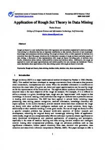
Fig. 4 Initial regions (a) and the final segmentation map after the region merging process (b) using the two criteria of feature similarity and spatial connectivity.

The region merging step in RCT takes into account both feature similarity and spatial relationship among regions. First, we identify the small segments whose number of pixels is less than a given threshold. From the experiments, we have found that the oversegmentation is considerably reduced by merging segments that have a number of pixels below 0.2% of the whole image size. Once we have identified all the small regions, they are fused with the most appropriate neighbor region. Such a region is one that is more similar in features and shares the greatest number of connected pixels. An example of this process is illustrated in Fig. 4. In Fig. 5, an example of the resultant images in each step of our method and the final segmented image are presented. In Figs. 5(a)–5(c), we can see the images of the feature channels using a, b and T, respectively. The presegmented image is shown in Fig. 5(d). Such an image is the result of the rough set–based segmentation, before the submission to the merging process. In this image, the borders of the segments detected are superimposed to the original image and we can observe that many small regions are present. The Fig. 5(e) shows the resultant segmentation of RCT after the merging process, where the oversegmentation issues were significantly reduced. In this image, we can see

that the pixels of the flower petals are associated in one segment despite the intensity differences of the red color. Moreover, the RCT method is able to clearly separate the red petals of the flower from the yellow center and the green background. 3 Experiments and Results The experiments conducted on images of natural scenes for the performance evaluation of our proposal are presented in this section. The evaluation is carried out by a thorough qualitative and quantitative analysis. Additionally, the assessment of RCT in comparison with other similar and recent state-of-the-art approaches is also presented. 3.1 Experimental Setup and RCT Parameter Selection For the evaluation of the RCT method, the scenario described by Yang et al.35 is replicated for the assessment of segmentation approaches. For these experiments, the Berkeley segmentation data set (BSD)36 is used. Such a data set is an empirical basis for segmentation algorithms evaluation. For each image, a ground-truth is available and may be used to quantify the reliability of a given method.

Fig. 5 Resulting images of the inner process. Feature components (a) a, (b) b, and (c) T , respectively. (d) The presegmented image before the region merging process and (e) the final-segmented image.

Journal of Electronic Imaging

023003-6

Mar–Apr 2014

•

Vol. 23(2)

Lizarraga-Morales et al.: Integration of color and texture cues in a rough set–based segmentation method

Moreover, the diversity of content of this data set, including landscapes, animals, buildings, and portraits, is a challenge for any segmentation algorithm. For a quantitative evaluation, four widely used metrics are adopted for the assessment of segmentation algorithms: Probabilistic Rand Index (PRI),37 Variation of Information (VoI),38 Global Consistency Error (GCE),36 and the Boundary Displacement Error (BDE).39 These measures provide a value obtained from the comparison of a segmented image and the corresponding ground-truth. For the estimation of these measures, we have used the MATLAB® source code made publicly available by Yang et al.35 Other performance measures for segmentation algorithms may be consulted in Table 1 of the article by Ilea and Whelan.3 The BDE measures the average displacement error between the boundary pixels of the segmented image and the closest boundary pixels in the ground-truth segmentations. The GCE evaluates the extent to which a segmentation map can be considered as a refinement of another segmentation. The VoI metric calculates conditional entropies between class labels distributions. The PRI counts the number of pixel pairs whose labels are consistent, both for the ground truth and for the segmentation result. If the test image and the ground truth images have no matches, the PRI is zero, its minimum value. The maximum value of 1 is achieved if the test image and all the segmentation references are identical. This measure is considered the most important in our evaluation because, as pointed out by Yang et al.,35 there is a good correlation between the PRI and human perception through the hand-labeled segmentations. For the PRI, the segmentation is considered better if the resulting value is closer to 1. For the other measures, the segmentation is superior if the values are closer to 0. Additionally to these widely used metrics, we have included the Normalized Probabilistic Rand index (NPR).37 The NPR, as it name indicates, is the normalization of the PRI in the range of ½−1; 1
. Its importance lies in the fact that it considers the differences among multiple ground-truth images through a nonuniform weighting of pixel pairs as a function

Table 1 Performance estimation of the RCT using different combinations of the parameters Ex and W . The performance is evaluated using the probabilistic Rand index (PRI). Ex∕W

3

5

7

9

11

50

0.7841

0.7848

0.7848

0.7847

0.7847

100

0.7843

0.7825

0.7844

0.7848

0.7847

150

0.7830

0.7844

0.7856

0.7769

0.7847

200

0.7826

0.7843

0.7747

0.7608

0.7848

250

0.7641

0.7830

0.7828

0.7746

0.7852

300

0.7603

0.7644

0.7704

0.7600

0.7660

350

0.7590

0.7650

0.7691

0.7480

0.7628

400

0.7593

0.7621

0.7690

0.7503

0.7551

Journal of Electronic Imaging

of the variability in the ground-truth set. Moreover, the NPR value is more sensitive to variations and it has a higher range of values than the PRI. As was previously mentioned, the parameters of a rough set–based segmentation method are ðW; ExÞ. In the approaches previously proposed18,23 using the RGB color space, the best couple of parameters according to the authors is (3, 100). In contrast, because the feature space used in this study has a different shape compared with the RGB color space, the most suitable parameters need to be estimated. The evaluation of the best combination of parameters is carried out using the 300 images taken from the BSD and quantitatively assessed using the PRI measure. We have exhaustively searched for the best window size W in the set f3; 5; 7; 9; 11g and the expanse Ex in the set of f50;100;150; : : : ; 400g. The influence of the fundamental parameters ðW; ExÞ on the performance of the RCT method is given in Table 1. The evaluations presented in this table are measured using the PRI. The expanse Ex is the similarity tolerance among the features used and W is the size of the neighborhood to analyze. The value of Ex has influence on the dilatation or contraction of the boundary region between the histogram and the histon, and therefore, on the value of the roughness index. If Ex is high, the association of similar pixels becomes more flexible, leading to undersegmentation issues. If Ex is small, the association becomes more rigid, making highly similar pixels to be considered as different regions, resulting in an oversegmentation. The parameter W has a direct impact on the computation time of the histon, since it defines the neighborhood size of the analysis for each pixel. It can be seen in Table 1 that the performance remains stable when Ex is small and the PRI starts to decrease when Ex ≥ 200. This decrement in the performance is caused by the fact that the ground-truth images from the BSD are, in general, undersegmented. Such fact has been also observed by Ilea and Whelan.15 The lowest PRI value of 0.7480 is obtained with the parameters (9, 350) and the best performance, PRI ¼ 0.7856, is found for (7, 150). Other parameters, like the value of d for the texture extraction and the weights in the Eq. (9), were also obtained in such exhaustive search. The window size d for the texture extraction was searched in the set d ¼ f1; 2; : : : ; 20g and the weights ωi in the set ωi ¼ f0; 0.1; : : : ; 1g. A window size of 21 × 21 pixles, meaning a d ¼ 10, and the set of weights ωi ¼ f0.2; 0.2; 0.6g have been found to provide the best results. 3.2 Performance Evaluation A quantitative evaluation of the RCT using the 300 images from the BSD was carried out. The distribution of the four quantitative measures PRI, VoI, GCE, and BDE are presented in Fig. 6. This figure shows the frequency that the RCT records a given value in each quantitative measure. For the PRI distribution [Fig. 6(a)], it is noteworthy the leaning of the PRI distribution to the maximum value of 1. This means that a high number of images achieve high PRI values, implying that the RCT method has a correspondence with the ground-truth. This figure also shows the tendency of the GCE [Fig. 6(c)] and BDE [Fig. 6(d)] distributions, where the tendency toward a error of zero is noticeable. The corresponding mean performance and the standard deviation

023003-7

Mar–Apr 2014

•

Vol. 23(2)

Lizarraga-Morales et al.: Integration of color and texture cues in a rough set–based segmentation method

Fig. 6 Distribution of the resulting values of the four measures for the Berkeley data set. For (a), a higher value is better, and for (b), (c), and (d), a small value is better. Table 2 Performance analysis of the RCT method using the five measures. Global Consistency Error (GCE)

Boundary Displacement Error (BDE)

Variation of Information (VoI)

Probabilistic Rand Index (PRI)

Normalized Probabilistic Rand Index

Mean (μ)

0.175

8.007

2.799

0.785

0.462

Std. Dev. (σ)

0.105

4.450

0.885

0.121

0.302

for each quantitative measure PRI, VoI, GCE, and BDE are shown in Table 2, where we have also added the NPR results. After the study of the performance of RCT, a comparison was conducted against other recent and similar approaches. The first comparison is carried out against the color-based technique using A-IFS histon.23 As previously mentioned, this method uses the RGB color representation. In the original A-IFS histon-based article, the average performance is assessed using only the PRI measure. The average performance reported for the A-IFS method is 0.7706, which is lower than the 0.785 index achieved by our RCT. This implies that the image representation in perceptual color spaces and the inclusion of texture information improves the performance of rough set–based methodologies. A comparison with three other state-of-the-art algorithms that use both color and texture features was carried out in our evaluation: the J-image segmentation (JSEG) method proposed by Deng andManjunath,40 the compression-based texture merging (CTM) approach introduced by Yang et al.,35 and the Clustering-based image Segmentation by Contourlet transform (CSC) presented by An and Pun.41 The average performance of each method using the four quantitative measures, PRI, BDE, GCE, and VoI, is Journal of Electronic Imaging

presented in Table 3. For the JSEG and the CTM approaches, the source codes provided at their web pages were downloaded and executed with the 300 BSD images. For the CSC method, the source code is not available; hence, the quantitative results presented in the original article are Table 3 Average performance and comparison with other methods. Within the parentheses is the number of images used by the authors for their evaluation. GCE

BDE

VoI

PRI

JSEG (300)

0.196

8.960

2.314

0.774

CTMγ¼0.1 (300)

0.176

9.421

2.464

0.756

CTMγ¼0.15 (300)

0.184

9.490

2.203

0.762

CTMγ¼0.2 (300)

0.187

9.896

2.023

0.761

CSC (100)

0.225

8.634

2.732

0.796

RCT (300)

0.175

8.007

2.799

0.785

023003-8

Mar–Apr 2014

•

Vol. 23(2)

Lizarraga-Morales et al.: Integration of color and texture cues in a rough set–based segmentation method

taken. It is important to highlight that the CSC evaluation, as mentioned in the original article,41 has been carried out using only a subset of 100 images from the complete set of 300 images from the BSD. This table shows that the best results for the GCE and the BDE measures are achieved by the proposed RCT method. The lowest value for the VoI measure is obtained by the CTM approach with γ ¼ 0.2. This means that our method is more accurate in relation to the ground-truth segmentations. For the PRI measure, the method RCT has obtained a 0.785 score, outperforming the JSEG (0.774) and CTM (0.761) approaches. The method that attains the highest PRI value is the CSC, reporting a result of 0.796 using only 100 images for the evaluation. Because mean results obtained by the RCT methodology and the CSC methodology are close to each other, a Student’s t-test was conducted to determine if the differences observed between the results are statistically significant. For a fair comparison between the two methods, we assume that both PRI distributions are normal and that there is not a significant difference between the standard deviations of the samples. However, no standard deviation is reported by CSC from the test samples. In this regard, the standard deviation from our results is used for both population samples. We also assume that the sample from CSC was selected randomly. Given those constrains, we calculate t using Eq. (15), μ − μ2 t ¼ q1ffiffiffiffiffiffiffiffiffiffiffiffiffiffi ; σ N11 þ N12

(15)

where μ1 ¼ 0.7961 is the mean results reported by CSC, μ2 ¼ 0.7852 is the mean result obtained by RCT, N 1 ¼ 100 is the number of segmentation tests in the sample by CSC, N 2 ¼ 300 is the number of segmentation tests in RCT sample, and σ ¼ 0.1209 is the standard deviation from our sample. The degrees of freedom for the t-test are df ¼ N 1 þ N 2 − 2 ¼ 398. The p-value obtained from t and df is P ¼ 0.4354. Because this value greatly differs from an acceptable significance level (e.g., 0.10, 0.05, 0.01), we conclude that the difference between the mean results reported by CSC and RCT is actually not statistically significant. Additionally to the Student’s t-test and in view that the authors of the CSC method do not define the selected subset of images used in their experiments, the tendency of the mean achieved by our RCT is analyzed for different subset

Fig. 7 Trend of the probabilistic Rand index measure mean achieved by the RCT method depending on the number of images taken from the Berkeley segmentation data set.

Journal of Electronic Imaging

sizes. For this analysis, we have taken the K ¼ f1; 2; : : : ; 300g images from the RCT results that achieve the best performance for the PRI measure. The PRI mean tendency is presented in Fig. 7, where it is shown that if the number of testing images is increased, the average performance decreases. In this figure, we can see that if 291 images are used, the RCT method achieves the mean performance of the CSC method of 0.796. Furthermore, if the best 100 images are taken for the RCT evaluation, our method achieves a mean PRI value of 0.8894, a much higher value than the 0.796 obtained by the CSC method that uses 100 images. A qualitative comparison of the segmentation results is presented in Fig. 8, where the first column corresponds to the CTM outcomes, the second column shows the resultant images of the JSEG method, and our RCT segmentations are shown in the third column. We only present qualitative comparisons of the methods whose results are available. In these examples, the edges of the segments are overlaid on the original image. From this qualitative comparison, we can observe that the RCT method is in general able to associate pixels with similar color and texture in single segments. For example in Fig. 8(a), there are oversegmentation issues in the outcomes of the CTM and JSEG methods. In Fig. 8(b), a challenging image is shown, since the color of the cheetah and its background are very similar. For this case, only the CTM and the RCT methods are able to separate the differences in texture of this image. In Fig. 8(c), the ability of RCT is noticeable for the association of the different intensities of blue in the sky, while the other methods separate them in two [Fig. 8(c2)] or even in three different segments [Fig. 8(c1)]. This ability can be also appreciated in Fig. 8(d), where the RCT is able to merge the elephants in only one segment. In the case of Figs. 8(e) and 8(f), the performance of the three methods is very similar. The last example shows how the CTM and the RCT succeed in the association of the pixels of the kangaroo while the JSEG attains an oversegmentation. Other color-texture segmentation algorithms that attain a high performance have been proposed, and they deserve a special mention. This is the case of the MIS method proposed by Krinidis and Pitas12 (PRI ¼ 0.79), the GSEG proposed by Garcia Ugarriza et al.6 (NPR ¼ 0.49), and the CTex method introduced by Ilea and Whelan15 (PRI ¼ 0.80). Despite the quantitative results of these methods, they have not been considered in this assessment because of the differences in the technical foundations between them and the RCT. The MIS method is spatially guided based in energy minimization and it is iterative in two stages of the method. The GSEG approach is also iterative and spatially guided. It uses a region growing technique and a multiresolution merging strategy, which might result in a considerable processing time. The CTex algorithm, although it is the method that attains the highest PRI value in the literature, has computational requirements that are considerably high due to its multiple steps and to the large number of distributions that have to be calculated during the adaptive spatial clustering process. The main attributes exhibited by our RCT are summarized. It is spatially blind: this means that it is not based on pixel-by-pixel agglomeration. In the RCT, the number of segments is automatically estimated without the need

023003-9

Mar–Apr 2014

•

Vol. 23(2)

Lizarraga-Morales et al.: Integration of color and texture cues in a rough set–based segmentation method

Fig. 8 A qualitative comparison of seven out of 300 segmentation outcomes between the CTM (first column), JSEG (second column), and our RCT (third column). The segmentation borders are overlaid on the original image.

Journal of Electronic Imaging

023003-10

Mar–Apr 2014

•

Vol. 23(2)

Lizarraga-Morales et al.: Integration of color and texture cues in a rough set–based segmentation method

of a predefined number of clusters or seeds initialization. It is able to integrate different kinds of features. The use of a perceptual color representation and the addition of textural features in a rough-set strategy achieves better results than other methods that use only color cues. Additionally, the significant peaks selection, jointly with the merging strategy, allows better results in comparison with other state-of-theart methods in terms of quantitative measures. 4 Conclusion In this article, the integration of color and visual texture cues in a rough set–based segmentation approach is proposed. The proposed method, named RCT, considers the spatial correlation and similarity of neighboring pixels, including information of separate color and texture channels. The computation of these features have been shown to be simple, yet they are representative of the image information. A thorough analysis of the performance of the RCT method showed that it can be successfully applied to natural image segmentation, where the resemblance to human perception may be desirable. Experiments on an extensive database show that our method yields better outcomes, outperforming other rough set–based approaches and state-of-the-art segmentation algorithms. Acknowledgments R.A. Lizarraga-Morales and F.E. Correa-Tome acknowledge the grants provided by the Mexican National Council of Science and Technology (CONACyT) and the Universidad de Guanajuato. References 1. L. Shapiro and G. Stockman, Computer Vision, Prentice-Hall, Upper Saddle River, New Jersey (2001). 2. T. Saarela and M. S. Landy, “Combination of texture and color cues in visual segmentation,” Vision Res. 58, 59–67 (2012). 3. D. E. Ilea and P. F. Whelan, “Image segmentation based on the integration of colour-texture descriptors—a review,” Pattern Recognit. 44(10–11), 2479–2501 (2011). 4. P. Nammalwar, O. Ghita, and P. F. Whelan, “Integration of feature distributions for color texture segmentation,” in Proc. 17th Int. Conf. Pattern Recognit., Vol. 1, pp. 716–719, IEEE, New York (2004). 5. K.-M. Chen and S.-Y. Chen, “Color texture segmentation using feature distributions,” Pattern Recognit. Lett. 23(7), 755–771 (2002). 6. L. Garcia Ugarriza et al., “Automatic image segmentation by dynamic region growth and multiresolution merging,” IEEE Trans. Image Process. 18(10), 2275–2288 (2009). 7. I. Fondón, C. Serrano, and B. Acha, “Color-texture image segmentation based on multistep region growing,” Opt. Eng. 45(5), 057002 (2006). 8. J. Angulo, “Morphological texture gradients. application to colour+texture watershed segmentation,” in Int. Symp. Math. Morphol., pp. 399– 410 (2007). 9. C. Meurie, A. Cohen, and Y. Ruichek, “An efficient combination of texture and color information for watershed segmentation,” in Image and Signal Processing, A. Elmoataz et al., Eds., pp. 147–156, Springer, Berlin, Heidelberg (2010). 10. S. Han et al., “Image segmentation based on grabcut framework integrating multiscale nonlinear structure tensor,” IEEE Trans. Image Process. 18(10), 2289–2302 (2009). 11. J. Kim and K. Hong, “Colour-texture segmentation using unsupervised graph cuts,” Pattern Recognit. 42(5), 735–750 (2009). 12. M. Krinidis and I. Pitas, “Color texture segmentation based on the modal energy of deformable surfaces,” IEEE Trans. Image Process. 18(7), 1613–1622 (2009). 13. M. Mignotte, “MDS-based segmentation model for the fusion of contour and texture cues in natural images,” Comput. Vision Image Understanding 116(9), 981–990 (2012). 14. W. S. Ooi and C. P. Lim, “Fuzzy clustering of color and texture features for image segmentation: a study on satellite image retrieval,” J. Intell. Fuzzy Syst. 17(3), 297–311 (2006). 15. D. E. Ilea and P. F. Whelan, “CTex—an adaptive unsupervised segmentation algorithm based on color-texture coherence,” IEEE Trans. Image Process. 17(10), 1926–1939 (2008).

Journal of Electronic Imaging

16. A. Mohabey and A. Ray, “Rough set theory based segmentation of color images,” in Fuzzy Inf. Process. Soc. NAFIPS 19th Int. Conf. North Am., pp. 338–342, IEEE, New York (2000). 17. Z. Pawlak, “Rough sets,” Int. J. Comput. Inf. Sci. 11(5), 341–356 (1982). 18. M. M. Mushrif and A. K. Ray, “Color image segmentation: rough-set theoretic approach,” Pattern Recognit. Lett. 29(4), 483–493 (2008). 19. N. I. Ghali, W. G. Abd-Elmonim, and A. E. Hassanien, “Object-based image retrieval system using rough set approach,” in Advances in Reasoning-Based Image Processing Intelligent Systems, R. Kountchev and K. Nakamatsu, Eds., Vol. 29, pp. 315–329, Springer, Berlin, Heidelberg (2012). 20. P. Chiranjeevi and S. Sengupta, “Robust detection of moving objects in video sequences through rough set theory framework,” Image Vision Comput. 30(11), 829–842 (2012). 21. S.-J. Hu and Z.-G. Shi, “A new approach for color text segmentation based on rough set theory,” in Proc. 3rd Int. Conf. Teach. Comput. Sci. (WTCS 2009), Y. Wu, Ed., Vol. 116, pp. 281–289, Springer, Berlin, Heidelberg (2012). 22. A. E. Hassanein et al., “Rough sets and near sets in medical imaging: a review,” IEEE Trans. Inf. Technol. Biomed. 13(6), 955–968 (2009). 23. M. M. Mushrif and A. K. Ray, “A-IFS histon based multithresholding algorithm for color image segmentation,” IEEE Signal Process. Lett. 16(3), 168–171 (2009). 24. L. Busin et al., “Color space selection for color image segmentation by spectral clustering,” in 2009 IEEE Int. Conf. Signal Image Process. Appl., pp. 262–267, IEEE, New York (2009). 25. M. Fairchild, Color Appearance Models, 2nd ed., Wiley, Hoboken, New Jersey (2005). 26. L. Lucchese and S. Mitray, “Color image segmentation: a state-of-theart survey,” in Proc. Indian Natl. Sci. Acad. (INSA-A). Delhi, India 67(2), 207–221 (2001). 27. P. Guo and M. Lyu, “A study on color space selection for determining image segmentation region number,” in Proc. Int. Conf. Artif. Intell., Vol. 3, pp. 1127–1132, CSREA Press, Las Vegas, Nevada (2000). 28. L. Busin, N. Vandenbroucke, and L. Macaire, “Color spaces and image segmentation,” Adv. Imaging Electron Phys. 151(7), 65–168 (2008). 29. F. Correa-Tome, R. Sanchez-Yanez, and V. Ayala-Ramirez, “Comparison of perceptual color spaces for natural image segmentation tasks,” Opt. Eng. 50(11), 117203 (2011). 30. L. Shafarenko, H. Petrou, and J. Kittler, “Histogram-based segmentation in a perceptually uniform color space,” IEEE Trans. Image Process. 7(9), 1354–1358 (1998). 31. T. Smith and J. Guild, “The C.I.E., colorimetric standards and their use,” Trans. Opt. Soc. 33(3), 73–134 (1932). 32. H. Cheng et al., “Color image segmentation: advances and prospects,” Pattern Recognit. 34(12), 2259–2281 (2001). 33. D.-C. Tseng and C.-H. Chang, “Color segmentation using perceptual attributes,” in Proc. 11th IAPR Int. Conf. Pattern Recognit., pp. 228–231, IEEE, New York (1992). 34. H. Cheng, X. Jiang, and J. Wang, “Color image segmentation based on homogram thresholding and region merging,” Pattern Recognit. 35(2), 373–393 (2002). 35. A. Y. Yang et al., “Unsupervised segmentation of natural images via lossy data compression,” Comput. Vision Image Understanding 110(2), 212–225 (2008). 36. D. Martin et al., “A database of human segmented natural images and its application to evaluation segmentation algorithms and measuring ecological statistics,” in Proc. 8th Int. Conf. Comput. Vision, Vol. 2, pp. 416–423, IEEE, New York (2001). 37. R. Unnikrishnan, C. Pantofaru, and M. Hebert, “Toward objective evaluation of image segmentation algorithms,” IEEE Trans. Pattern Anal. Machine Intell. 29(6), 929–944 (2007). 38. M. Meila, “Comparing clusterings-an information based distance,” J. Multivar. Anal. 98, 873–895 (2007). 39. J. Freixenet et al., “Yet another survey on image segmentation: region and boundary information integration,” in Computer Vision ECCV 2002, A. Heyden et al., Eds., Lecture Notes in Computer Science, Vol. 2352, pp. 408–422, Springer, Berlin, Heidelberg (2002). 40. Y. Deng and B. Manjunath, “Unsupervised segmentation of color-texture regions in images and video,” IEEE Trans. Pattern Anal. Mach. Intell. 23, 800–810 (2001). 41. N.-Y. An and C.-M. Pun, “Color image segmentation using adaptive color quantization and multiresolution texture characterization,” Signal Image Video Process., 1–12 (2012). Rocio A. Lizarraga-Morales received her BEng degree in electronics in 2005 from the Instituto Tecnológico de Mazatlán and her MEng degree in electrical engineering in 2009 from the Universidad de Guanajuato, Mexico. She is currently working toward her DEng degree, also at the Universidad de Guanajuato. Her current research interests include image and signal processing, pattern recognition, and computer vision.

023003-11

Mar–Apr 2014

•

Vol. 23(2)

Lizarraga-Morales et al.: Integration of color and texture cues in a rough set–based segmentation method Raul E. Sanchez-Yanez concluded his studies of Doctor of Science (optics) at the Centro de Investigaciones en Óptica (Leon, Mexico) in 2002. He also has a MEng degree in electrical engineering and a BEng in electronics, both from the Universidad de Guanajuato, where he has been a tenure track professor since 2003. His main research interests include color and texture analysis for computer vision tasks and the computational intelligence applications in feature extraction and decision making. Victor Ayala-Ramirez received his BEng in electronics and the MEng in electrical engineering from the Universidad de Guanajuato in 1989 and 1994, respectively, and the PhD degree in industrial computer

Journal of Electronic Imaging

science from Université Paul Sabatier (Toulouse, France) in 2000. He has been a tenure track professor at the Universidad de Guanajuato, Mexico, since 1993. His main research interest is the design and development of soft computing techniques for applications in computer vision and mobile robotics. Fernando E. Correa-Tome received his MEng in electrical engineering in 2011 and his BEng in communications and electronics in 2009, from the Universidad de Guanajuato, Mexico. His current research interests include image and signal processing, machine learning, pattern recognition, computer vision, algorithms, and data structures.

023003-12

Mar–Apr 2014

•

Vol. 23(2)